Following Friedmans permanent income hypothesis, we may write Y i = α + βX i where Y i = permanent consumption expenditure and X i

Following Friedman€™s permanent income hypothesis, we may write

Y^ˆ—_i = α + βX^ˆ—_i

where Y^ˆ—_i = €œpermanent€ consumption expenditure and X^ˆ—_i = €œpermanent€ income. Instead of observing the €œpermanent€ variables, we observe

Y_i = Y^*_i + u_i

X_i = X^*_i + v_i

where Y_i and X_i are the quantities that can be observed or measured and where u_i and v_i are measurement errors in Y^ˆ— and X^ˆ—, respectively. Using the observable quantities, we can write the consumption function as

Y_i = α + β(X_i €“ v_i) + u_i

= α + βX_i + (u_i €“ βv_i)

Assuming that (1) I(u_i) = E(v_i) = 0, (2) var (u_i) = σ²_u and var (v_i) = σ²_v, (3) cov (Y^*_i, u_i) = 0, cov (X^*_i, v_i) = 0, and (4) cov (u_i, X_i^*) = cov (v_i, Y^*_i) = cov (u_i, v_i) = 0, show that in large samples β estimated from Eq. (2) can be expressed as

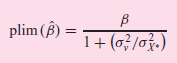
a. What can you say about the nature of the bias in β̂?

b. If the sample size increases indefinitely, will the estimated β tend toward equality with the true β?

plim () = 1+ (0} /of.) 1+ (a/a}.)