Repeat Exercise 6.20 but refer to the demand for personal computers given in the following equation. Is there a difference between the estimated income elasticities for cell phones and personal computers? If so, what factors might account for the difference?

YÌ‚_i = -6.5833 + 0.0018X_i

In exercise 6.20

The following table gives data on the number of cell phone subscribers and the number of personal computers (PCs), both per 100 persons, and the purchasing power adjusted per capita income in dollars for a sample of 34 countries. Thus we have cross-sectional data. These data are for the year 2003 and are obtained from the Statistical Abstract of the United states, 2006.

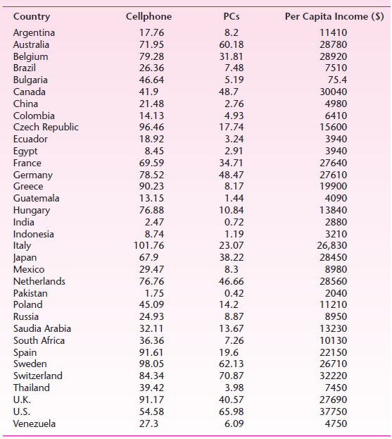
Although cell phones and personal computers are used extensively in the United States, that is not the case in many countries. To see if per capita income is a factor in the use of cell phones and PCs, we regressed each of these means of communication on per capita income using the sample of 34 countries. The results are as follows: 

Demand for Cell Phones. Letting Y = number of cell phone subscribers and X = purchasing-power-adjusted per capita income, we obtained the following  regression.

         YÌ‚_i = 14.4773 + 0.0022X_i

se (β̂₁) = 6.1523;se (β̂₂) = 0.00032

        r² = 0.6023

The slope coefficient suggests that if per capita income goes up by, say, $1,000, on average, the number of cell phone subscribers goes up by about 2.2 per 100 persons. The intercept value of about 14.47 suggests that even if the per capita income is zero, the average number of cell phone subscribers isabout 14 per 100 subscribers. Again, this  interpretation may not have much meaning, for in our sample we do not have any country with zero per capita income. The r 2 value is moderately high. But notice that our sample includes a variety of countries with varying levels of income. In such a diverse sample we would not expect a very high r 2 value.
After we study Chapter 5, we will show how the estimated standard errors reported in Equation 3.7.3 can be used to assess the statistical significance of the estimated coefficients.

Demand for Personal Computers. Although the prices of personal computers have come down substantially over the years, PCs are still not ubiquitous. An important determinant of the demand for personal computers is personal income. Another determinant is price, but we do not have comparative data on PC prices for the countries in our sample.
Letting Y denote the number of PCs and X the per capita income, we have the following €œpartial€ demand for the PCs (partial because we do not have comparative price data or data on other variables that might affect the demand for the PCs).

        YÌ‚_i = -3.5833 + 0.0018X_i

se (β̂₁) = 2.7437;se (β̂₂) = 0.00014

        r² = 0.8290

As these results suggest, per capita personal income has a positive relationship to the demand for PCs. After we study Chapter 5, you will see that, statistically, per capita personal income is an important determinant of the demand for PCs. The negative value of the intercept in the present instance has no practical significance. Despite the diversity of our sample, the estimated r² value is quite high. The interpretation of the slope coefficient is that if per capita income increases by, say, $1,000, on average, the demand for personal computers goes up by about 2 units per 100 persons.
Even though the use of personal computers is spreading quickly, there are many countries which still use main-frame computers. Therefore, the total usage of computers in those countries may be much higher than that indicated by the sale of PCs.

Required

a. Plot cell phone demand against purchasing power (PP) adjusted per capita income.
b. Plot the log of cell phone demand against the log of PP-adjusted per capita income.
c. What is the difference between the two graphs?
d. From these two graphs, do you think that a double-log model might provide a better fit to the data than the linear model? Estimate the double-log model.
e. How do you interpret the slope coefficient in the double-log model?
f. Is the estimated slope coefficient in the double-log model statistically significant at the 5% level?

g. How would you estimate the elasticity of cell phone demand with respect to PPadjusted income for the linear model given in Eq. (3.7.3)? What additional information, if any, do you need? Call the estimated elasticity the income elasticity.
h. Is there a difference between the income elasticity estimated from the double-log model and that estimated from the linear model? If so, which model would you choose?

Transcribed Image Text:

Cellphone Per Capita Income ($) Country PCs Argentina Australia 17.76 8.2 11410 71.95 60.18 28780 Belgium Brazil Bulgaria Canada 31.81 79.28 28920 26.36 7.48 7510 46.64 41.9 75.4 5.19 48.7 30040 China 4980 21.48 2.76 Colombia 14.13 96.46 4.93 6410 Czech Republic Ecuador Egypt France Germany Greece 17.74 15600 3940 18.92 3.24 2.91 3940 8.45 34.71 69.59 27640 78.52 48.47 27610 90.23 8.17 19900 Guatemala Hungary India 13.15 1.44 4090 76.88 10.84 13840 0.72 2.47 2880 Indonesia 8.74 1.19 3210 Italy Japan 101.76 23.07 38.22 26,830 67.9 28450 8.3 Mexico 29.47 8980 Netherlands 76.76 46.66 28560 Pakistan Poland 1.75 0.42 2040 45.09 14.2 11210 8.87 Russia 24.93 8950 Saudia Arabia South Africa 32.11 13.67 13230 36.36 7.26 10130 Spain Sweden 91.61 19.6 22150 98.05 62.13 26710 Switzerland 70.87 84.34 32220 Thailand 39.42 3.98 7450 U.K. 91.17 40.57 27690 U.S. 37750 54.58 65.98 Venezuela 6.09 27.3 4750