The regression shown in column (2) was estimated again, this time using data from 1992 (4000 observations selected at random from the March 1993 Current Population Survey, converted into 2015 dollars using the Consumer Price Index). The results are

\(\widehat{A H E}=1.30+8.94\) College - 4.38 Female +0.67 Age, \(S E R=9.88, \bar{R}^{2}=0.21\).

\(\begin{array}{lll}(1.65) & (0.34) \quad(0.30) \quad(0.05)\end{array}\)

Comparing this regression to the regression for 2015 shown in column (2), was there a statistically significant change in the coefficient on College?

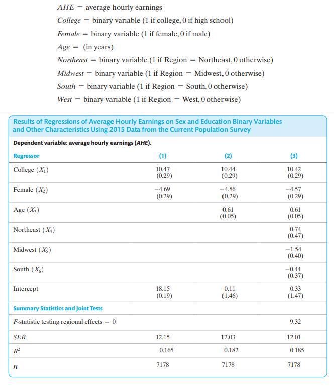
AHE average hourly earnings College = binary variable (1 if college, 0 if high school) Female = binary variable (1 if female,0 if male) Age = (in years) Northeast = binary variable (1 if Region = Northeast, 0 otherwise) Midwest = binary variable (1 if Region Midwest, 0 otherwise) South = binary variable (1 if Region = South, 0 otherwise) West = binary variable (1 if Region = West, 0 otherwise) Results of Regressions of Average Hourly Earnings on Sex and Education Binary Variables and Other Characteristics Using 2015 Data from the Current Population Survey Dependent variable: average hourly earnings (AHE). Regressor (1) College (X1) Female (X2) Age (X3) Northeast (X4) Midwest (X's) (2) (3) 10.47 10.44 10.42 (0.29) (0.29) (0.29) -4.69 -4.56 (0.29) (0.29) -4.57 (0.29) 0.61 (0.05) 0.61 (0.05) 0.74 (0.47) -1.54 (0.40) South (X) -0.44 (0.37) Intercept 18.15 0.11 (0.19) (1.46) 0.33 (1.47) Summary Statistics and Joint Tests F-statistic testing regional effects =0 9.32 SER 12.15 12.03 12.01 R 0.165 0.182 0.185 7178 7178 7178 n