Plot contours of the maximum principal stress 1 in Exercise 3.8 in the region 0

Plot contours of the maximum principal stress σ₁ in Exercise 3.8 in the region 0 ≤ x ≤ L, – c ≤ y≤ c, with L = 1, c = 0.1, and P = 1.

Data from exercise 3.8

Exercise 8.2 provides the plane stress (see Exercise 3.5) solution for a cantilever beam of unit thickness, with depth 2c, and carrying an end load of P with stresses given by: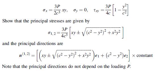

Data from exercise 8.2

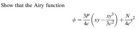
solves the following cantilever beam problem, as shown in the following figure. As usual for such problems, boundary conditions at the ends (x = 0 and L) should be formulated only in terms of the resultant force system, while at y = ± c the exact pointwise specification should be used. For the case with N = 0, compare the elasticity stress field with the corresponding results from strength of materials theory.

Data from exercise 3.5

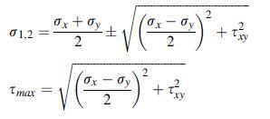
A two-dimensional state of plane stress in the x, y-plane is defined by σ_z = τ _yz = τ _zx = 0. Using general principal value theory, show that for this case the in-plane principal stresses and maximum shear stress are given by:

Transcribed Image Text:

0x = 3P 3P 2c3, dy = 0, Tay 4c Show that the principal stresses are given by 1,25 - xy+(c- y2)+xy 3P 463 and the principal directions are 1 = [ (xy (c y) + x3) e + (c - y) ] Note that the principal directions do not depend on the loading P. X constant