This exercise is based on data describing recreation visits to 17 beaches in the American state of North Carolina by a sample of residents from the eastern part of the state. The dataset NC_beach (available on the book’s website) was collected by John Whitehead and colleagues, and an analysis based on these data is provided by Whitehead et al. (2010). Here we use a configuration of the data that is designed to examine single and multiple equation count data models.
We observe 610 people who made at least one trip to visit a beach (and no more than 50 trips) in the southeastern part of North Carolina in 2003. The dataset contains the following variables:
id – unique identifier for each household inc – annual household income tr₁, tr₂,… – trips to each of the 17 beaches pr₁, pr₂,… – travel costs for each of the 17 beaches width₁, width₂,… – width (in feet) of each of the 17 beaches park₁, park₂,… – number of parking spaces (in 100s) available at each of the 17 beaches.
Travel costs were computed using $0.37 per mile for out-of-pocket costs, and one-third the average wage rate for the opportunity cost of travel time. The width and park variables are site attributes that are constant across individuals. Data files are also available that link the names of the beaches to an index number, which references each beach to its trip, travel cost, and site attribute variables. Using these data complete the following:

(a) Wrightsville Beach (#10) is the most frequented destination.
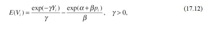
Estimate a single-demand equation for trips to this beach using the Poisson model, exploring versions that include and then exclude income as an explanatory variable. Depending on your findings, use the indirect utility function in Eq. (17.12) or (17.13) to estimate the average welfare loss in the sample if the site were eliminated. Then estimate the average annual welfare loss from a $5 per person beach access fee.

Eq (17.12)

Eq (17.13)

(b) Consider now a system of 17 demand equations for trips. Estimate models of the form

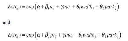
Report the coefficient estimates, their statistical significance, and interpret their signs and magnitudes. Note any differences you find when you estimate a single price coefficient versus 17 different price coefficients. What might explain these differences?

(c) Repeat part (b) using the natural log of width. Interpret the coefficient estimate and comment on the differences you find with the linear in width specification. Use the model with the separate price coefficients and log specification to estimate the welfare effects in increasing beach width 50 percent at Wrightsville and Carolina Beaches.

(d) Note that a model of the form

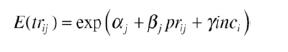
can be estimated, but it does not allow direct inclusion of the site varying characteristics. Estimate this model to recover α1,...,αJ, and then examine the correlation between the constants and beach width by running the regression

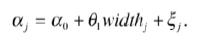
Consider also a similar regression using the log of width. Compare your point estimates to what you find in parts (b) and (c), and discuss the extent to which you think the estimates of the site attribute coefficients in the earlier models are well identified.

Transcribed Image Text:

E(V)= exp(-) Y exp(a + Bp;) Y>0, (17.12)