

An APT model is based on two independent systematic factors (F_{1}) and (F_{2}), both with zero expected
Question:
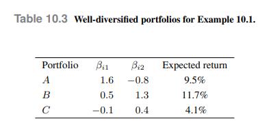
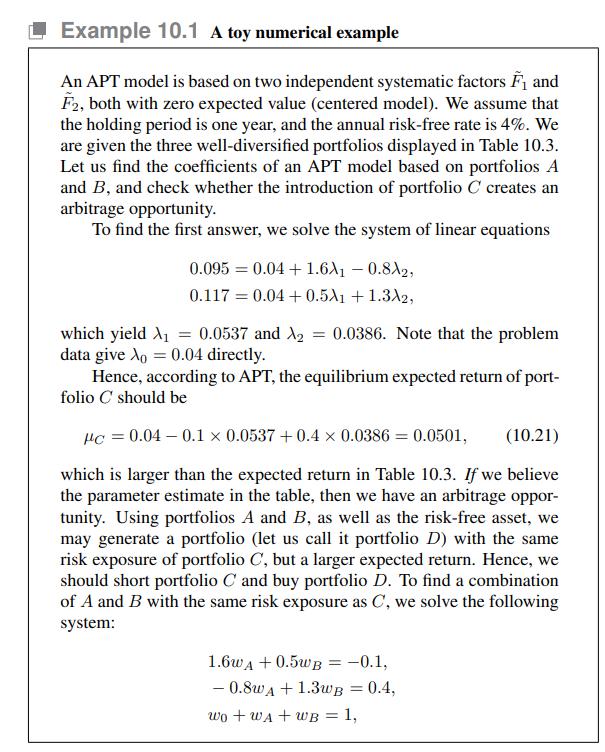
An APT model is based on two independent systematic factors \(F_{1}\) and \(F_{2}\), both with zero expected value (centered model). We assume that the holding period is one year, and the annual risk-free rate is \(4 \%\). We are given the three well-diversified portfolios displayed in Table 10.3. Let us find the coefficients of an APT model based on portfolios \(A\) and \(B\), and check whether the introduction of portfolio \(C\) creates an arbitrage opportunity.
To find the first answer, we solve the system of linear equations
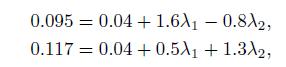
which yield ![]() =0.0537, and
=0.0537, and![]() =0.0386. Note that the problem data give
=0.0386. Note that the problem data give ![]() =0.04 directly.
=0.04 directly.
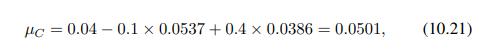
Hence, according to APT, the equilibrium expected return of portfolio \(C\) should be
![]()
which is larger than the expected return in Table 10.3. If we believe the parameter estimate in the table, then we have an arbitrage opportunity. Using portfolios \(A\) and \(B\), as well as the risk-free asset, we may generate a portfolio (let us call it portfolio \(D\) ) with the same risk exposure of portfolio \(C\), but a larger expected return. Hence, we should short portfolio \(C\) and buy portfolio \(D\). To find a combination of \(A\) and \(B\) with the same risk exposure as \(C\), we solve the following system:
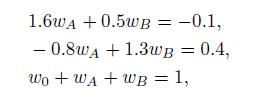
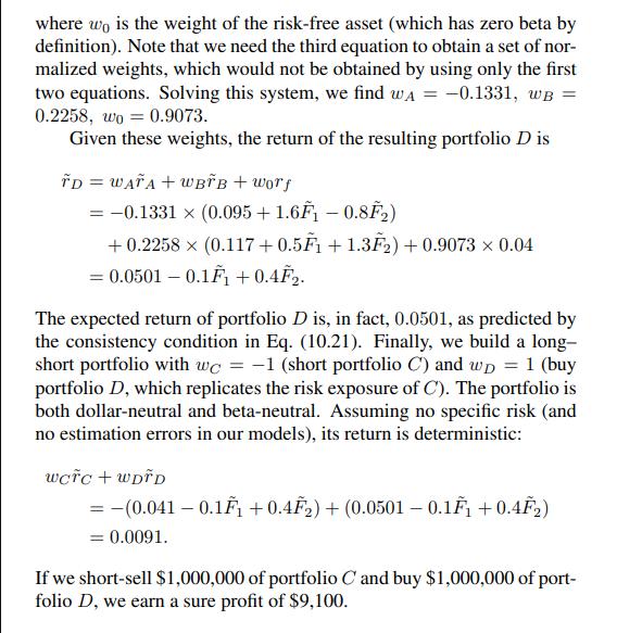
where \(w_{0}\) is the weight of the risk-free asset (which has zero beta by definition). Note that we need the third equation to obtain a set of normalized weights, which would not be obtained by using only the first two equations. Solving this system, we find \(w_{A}=0.1331 w_{B}=\) \(0.2258 w_{0}=0.9073\).
Given these weights, the return of the resulting portfolio \(D\) is 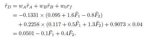
The expected return of portfolio \(D\) is, in fact, 0.0501, as predicted by the consistency condition in Eq. (10.21). Finally, we build a long short portfolio with \(w_{C}=1\) (short portfolio \(C\) ) and \(w_{D}=1\) (buy portfolio \(D\), which replicates the risk exposure of \(C\) ). The portfolio is both dollar-neutral and beta-neutral. Assuming no specific risk (and no estimation errors in our models), its return is deterministic: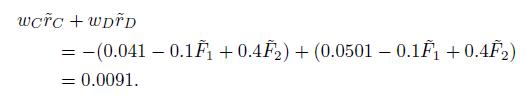
If we short-sell \(\$ 1,000,000\) of portfolio \(C\) and buy \(\$ 1,000,000\) of portfolio \(D\), we earn a sure profit of \(\$ 9,100\).
Data From Equation (10.21)
Data From Table 10.3
Data From Example 10.1
Step by Step Answer:


An Introduction To Financial Markets A Quantitative Approach
ISBN: 9781118014776
1st Edition
Authors: Paolo Brandimarte
