Annuities are assets that provide a stream of periodic payments over a period of time. This may correspond to the buyer's lifetime in the case of life insurances and pension funds in the decumulation phase (when the accumulated wealth is depleted in order to provide pension payments). Pricing an annuity under longevity risk requires tools from actuarial mathematics. Furthermore, the long time span involved implies considerable uncertainty about future interest rates. The picture may be further complicated if the annuity is inflation-indexed.

Here, we consider a simple annuity providing fixed payments over a given time horizon, disregarding interest rate risk. Such an annuity is just a bond whereby no face value is redeemed, and it may be priced given a term structure of interest rates. It is useful to find an explicit formula, under the further simplification of a flat term structure, e.g., for a given annually compounded yield:

\[r_{1}\left(t T_{i}\right)=y_{1}\]

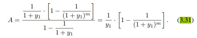
where \(T_{i}, i=1 \quad m\), is the set of time instants at which a payment is made. Using \(y_{1}\) makes sense if we consider annual payments (in practice, typical annuities involve monthly payments). The price of a unit annuity, paying \(\$ 1\) at each relevant epoch, is

\[A=\underbrace{m}_{i=1} \frac{1}{\left(1+y_{1}\right)^{i}}\]

We may find a compact expression for this value, by relying on the geometric series and using the same trick as in Example 3.3. If we consider 

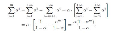
Plugging 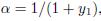 we find

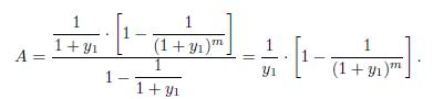
It is important to see the connection between this formula and Eq. (3.3). In that case, we have cash flows \(L\) at times \(t=0 \quad T \quad 1\), and we are evaluating the terminal wealth \(W_{T}\) at time \(T\). Here, we have cash flows \(C=1\) at times \(t=1 \quad T\), and we are evaluating the annuity \(A\) at time \(t=0\). To see the equivalence, we can shift \(W_{T}\) backward in time by \(T+1\) time periods, to time \(t=0\). This requires dividing Eq. (3.3) by \(\left(1+y_{1}\right)^{T+1}\) :

which is consistent with Eq. (3.31).

Data From Equation 3.31

Transcribed Image Text:

(0, 1)