Consider a countercurrent mass-transfer device for which the equilibrium distribution relation consists of a set of discrete values \(\left\{X_{i D}, Y_{i D}\right\}\) instead of a continuous model such as Henry's law. An analysis similar to that presented in Example 3.13 is still possible using the cubic spline interpolation capabilities of Mathcad. Cubic spline interpolation passes a smooth curve through a set of points in such a way that the first and second derivatives are continuous across each point. Once the cubic spline describing a data set is assembled, it can be used as if it were a continuous model relating the two variables to predict accurately interpolated values. It can also be derived or integrated numerically as needed. For the case of transfer from phases \(V\) to \(L\) and a concave-downward equilibrium curve described by the data set \(\left\{X_{i D}, Y_{i D}\right\}\), the procedure in Mathcad is as follows:

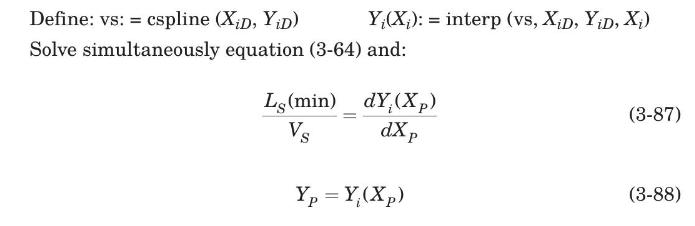
[In equation (3-87), the first-derivative operator is from Operators list on the Math tab of Mathcad (Maxfield, 2014).]

Write a Mathcad program to solve equations (3-64), (3-87), and (3-88) and test it with data from the adsorber of Example 3.12.

Data From Example 3.13:-

Consider an absorber or stripper in which the equilibrium is described by Henry’s
law: yi = mxi. It is easy to show that the equilibrium-distribution curve in terms of
mol ratios is given by 

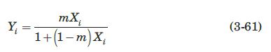
The general behavior of the XY distribution curve can be ascertained, for different
values of m, by means of the first and second derivatives of equation (3-49): 

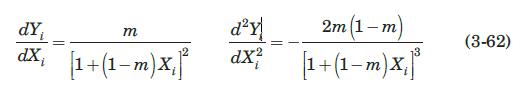
The sign of the second derivative will depend on the value of m. If m 1.0, the second derivative will be positive for all values of Xi and the equilibrium-distribution curve will always be concave upward; therefore, the operating line that gives the minimum vapor rate for a stripper will be tangent to the equilibrium curve at some point P(XP, YP) in the interval Xout

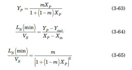
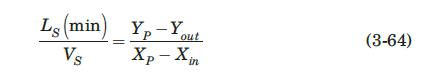
Equations (3-63) and (3-64) arise from the fact that the tangent point P is located on both the equilibrium curve and the operating line. Equation (3-65) states that, at the tangent point P, the slope of the equilibrium line equals the slope of the operating line. Consider now a stripper with known values of m (>1.0), LS, Xin, Yin, and Xout. The coordinates of the tangent point and the minimum gas flow rate, VS(min), are determined by simultaneously solving equation (3-63) and

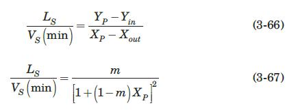
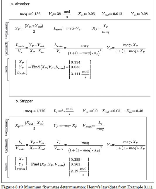
Figure 3.19 shows a Mathcad program to implement the solution of equations (3-63), (3-64), and (3-65) for an absorber, and equations (3-63), (3-66), and (3-67) for a stripper. For comparison purposes, the program uses data, where the minimum flow rates were determined by a graphical method. The results 

Figure 3.19:-

Data From Example 3.12:-

Nitrogen dioxide, NO₂, produced by a thermal process for fixation of nitrogen, is to be removed from a dilute mixture with air by adsorption on silica gel in a continuous countercurrent adsorber. The mass flow rate of the gas entering the adsorber is 0.50 kg/s; it contains 1.5% NO₂ by volume, and 85% of the NO₂ is to be removed. Operation is to be isothermal at 298 K and 1 atm. The entering gel will be free of NO₂. If twice the minimum gel rate is to be used, calculate the gel mass flow rate and the composition of the gel leaving the process. The equilibrium adsorption data for this system at this temperature are from Treybal (1980).

Equation 3-64:-

Transcribed Image Text:

Define: vs: cspline (XD, YiD) Y(X): interp (vs, XiD, YiD, X) Solve simultaneously equation (3-64) and: = Ls (min) dY,(XP) Vs dX P Yp=Y(Xp) (3-87) (3-88)