CRR model with dividends (2). We consider a riskless asset priced as

\[ S_{k}^{(0)}=S_{0}^{(0)}(1+r)^{k}, \quad k=0,1, \ldots, N \]

with \(r>-1\), and a risky asset \(S^{(1)}\) whose return is given by

\[ R_{k}:=\frac{S_{k}^{(1)}-S_{k-1}^{(1)}}{S_{k-1}^{(1)}}, \quad k=1,2, \ldots, N \]

with \(N+1\) time instants \(k=0,1, \ldots, N\) and \(d=1\). In the CRR model the return \(R_{k}\) is random and allowed to take two values \(a\) and \(b\) at each time step, i.e.
\[ R_{k} \in\{a, b\}, \quad k=1,2, \ldots, N \]
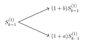
with \(-1(1+b) S_{k-1}^{(1)} & \text { if } R_{k}=b \tag{3.52}\\
(1+a) S_{k-1}^{(1)} & \text { if } R_{k}=a \end{array}ight\}=\left(1+R_{k}ight) S_{k-1}^{(1)}, \quad k=1,2, \ldots, N \]
according to the tree

and we have \[
S_{k}^{(1)}=S_{0}^{(1)} \prod_{i=1}^{k}\left(1+R_{i}ight), \quad k=0,1, \ldots, N \]
The information \(\mathcal{F}_{k}\) known to the market up to time \(k\) is given by the knowledge of \(S_{1}^{(1)}, S_{2}^{(1)}, \ldots, S_{k}^{(1)}\), i.e. we write \[
\mathcal{F}_{k}=\sigma\left(S_{1}^{(1)}, S_{2}^{(1)}, \ldots, S_{k}^{(1)}ight)=\sigma\left(R_{1}, R_{2}, \ldots, R_{k}ight)
\]
\(k=0,1, \ldots, N\), where \(S_{0}^{(1)}\) is a constant and \(\mathcal{F}_{0}=\{\emptyset, \Omega\}\) contains no information.

Under the risk-neutral probability measure \(\mathbb{P}^{*}\) defined by \[
p^{*}:=\mathbb{P}^{*}\left(R_{k}=bight)=\frac{r-a}{b-a}>0, \quad q^{*}:=\mathbb{P}^{*}\left(R_{k}=aight)=\frac{b-r}{b-a}>0, \]
\(k=1,2, \ldots, N\), the asset returns \(\left(R_{k}ight)_{k=1,2, \ldots, N}\) form a sequence of independent identically distributed random variables.
In what follows we assume that the stock \(S_{k}\) pays a dividend rate \(\alpha>0\) at times \(k=\) \(1,2, \ldots, N\). At the beginning of every time step \(k=1,2, \ldots, N\), the price \(S_{k}\) is immediately adjusted to its ex-dividend level by losing \(\alpha \%\) of its value. The following ten questions are interdependent and should be treated in sequence.

a) Rewrite the evolution (3.52) of \(S_{k-1}^{(1)}\) to \(S_{k}^{(1)}\) in the presence of a daily dividend rate \(\alpha>0\).

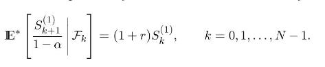
b) Express the dividend amount as a percentage of the ex-dividend price \(S_{k}^{(1)}\), and show that under the risk-neutral probability measure the return of the risky asset satisfies

c) We consider a (predictable) portfolio strategy \(\left(\xi_{k}, \eta_{k}ight)_{k=1,2, \ldots, N}\) with value process \[
V_{k}=\xi_{k+1} S_{k}^{(1)}+\eta_{k+1} S_{k}^{(0)}
\]
at time \(k=0,1, \ldots, N-1\). Write down the self-financing condition for the portfolio value process \(\left(V_{k}ight)_{k=0,1, \ldots, N}\) by taking into account the reinvested dividends, and give the expression of \(V_{N}\).

d) Show that under the self-financing condition, the discounted portfolio value process \[
\tilde{V}_{k}:=\frac{V_{k}}{S_{k}^{(0)}}, \quad k=0,1, \ldots, N \]
is a martingale under the risk-neutral probability measure \(\mathbb{P}^{*}\).

e) Show that the price at time \(k=0,1, \ldots, N\) of a claim with random payoff \(C\) can be written as \[
V_{k}=\frac{1}{(1+r)^{N-k}} \mathbb{E}^{*}\left[C \mid \mathcal{F}_{k}ight], \quad k=0,1, \ldots, N \]
assuming that the claim \(C\) is attained at time \(N\) by the portfolio strategy \(\left(\xi_{k}, \eta_{k}ight)_{k=1,2, \ldots, N}\).

f) Compute the price at time \(t=0,1, \ldots, N\) of a vanilla option with payoff \(h\left(S_{N}^{(1)}ight)\) using the pricing function \[
\begin{aligned}
& C_{0}(k, x, N,

a, b, r) \\
& \quad:=\frac{1}{(1+r)^{N-k}} \sum_{l=0}^{N-k}\left(\begin{array}{c}
N-k \\
l \end{array}ight)\left(p^{*}ight)^{l}\left(q^{*}ight)^{N-k-l} h\left(x(1+b)^{l}(1+a)^{N-k-l}ight)
\end{aligned}
\]
of a vanilla claim with payoff \(h\left(S_{N}^{(1)}ight)\).

g) Show that the price at time \(t=0,1, \ldots, N\) of a vanilla option with payoff function \(h\left(S_{N}^{(1)}ight)\) can be rewritten as \[
V_{k}=C_{\alpha}\left(k, S_{k}^{(1)}, N, a_{\alpha}, b_{\alpha}, r_{\alpha}ight):=(1-\alpha)^{N-k} C_{0}\left(k, S_{k}^{(1)}, N, a_{\alpha}, b_{\alpha}, r_{\alpha}ight), \]
\(k=0,1, \ldots, N\), where the coefficients \(a_{\alpha}, b_{\alpha}, r_{\alpha}\) will be determined explicitly.
h) Find a recurrence relation between the functions \(C_{\alpha}\left(k, x, N, a_{\alpha}, b_{\alpha}, r_{\alpha}ight)\) and \(C_{\alpha}(k+\) \(\left.1, x, N, a_{\alpha}, b_{\alpha}, r_{\alpha}ight)\) using the martingale property of the discounted portfolio value process \(\left(\widetilde{V}_{k}ight)_{k=0,1, \ldots, N}\) under the risk-neutral probability measure \(\mathbb{P}^{*}\).
i) Using the function \(C_{0}\left(k, x, N, a_{\alpha}, b_{\alpha}, r_{\alpha}ight)\), compute the quantity \(\xi_{k}\) of risky asset \(S_{k}^{(1)}\) allocated on the time interval \([k-1, k)\) in a self-financing portfolio hedging the claim \(C=h\left(S_{N}^{(1)}ight)\).

j) How are the dividends reinvested in the self-financing hedging portfolio?

Transcribed Image Text:

S(1) k-1 (1+b)S() k-1 *(1 +a)S() k-1