CRR model with transaction costs (Boyle and Vorst (1992), Mel'nikov and Petrachenko (2005)). Stock broker income is generated by commissions or transaction costs representing the difference between ask prices (at which they are willing to sell an asset to their client), and bid prices (at which they are willing to buy an asset from their client).

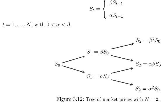
We consider a discrete-time Cox-Ross-Rubinstein model with one risky asset priced \(S_{t}\) at time \(t=0,1, \ldots, N\). The price \(A_{t}\) of the riskless asset evolves as

\[
A_{t}=ho^{t}, \quad t=0,1, \ldots, N \]
with \(A_{0}:=1\) and \(ho>0\), and the random evolution of \(S_{t-1}\) to \(S_{t}\) is given by two possible returns \(\alpha, \beta\) as

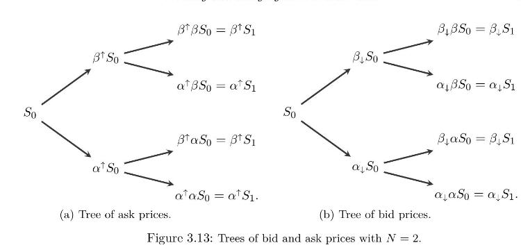
The ask and bid prices of the risky asset quoted \(S_{t}\) on the market are respectively given by \((1+\lambda) S_{t}\), and \((1-\lambda) S_{t}\) for some \(\lambda \in[0,1)\), such that \[
\left\{\begin{array}{l}
\alpha^{\uparrow}:=\alpha(1+\lambda)\alpha_{\downarrow}:=\alpha(1-\lambda)\alpha^{\uparrow}:=\alpha(1+\lambda)\end{array}ight.
\]
i.e. transaction costs are charged at the rate \(\lambda \in[0,1)\), proportionally to the traded amount.

The riskless asset is not subject to transaction costs or bid/ask prices and is priced \(A_{t}\) at time \(t=0,1, \ldots, N\). We consider a predictable, self-financing replicating portfolio strategy \[
\left(\eta_{t}\left(S_{t-1}ight), \xi_{t}\left(S_{t-1}ight)ight)_{t=1,2, \ldots, N}
\]
made of \(\eta_{t}\left(S_{t-1}ight)\) of the riskless asset \(A_{t}\) and of \(\xi_{t}\left(S_{t-1}ight)\) units of the risky asset \(S_{t}\) at time \(t=1,2, \ldots, N\).
Our goal is to derive a backward recursion giving \(\xi_{t}\left(S_{t-1}ight), \eta_{t}\left(S_{t-1}ight)\) from \(\xi_{t+1}\left(S_{t}ight), \eta_{t+1}\left(S_{t}ight)\) for \(t=N-1, N-2 \ldots, 1\). The following questions are interdependent and should be treated in sequence.

a) We consider a portfolio reallocation \(\left(\eta_{t}\left(S_{t-1}ight), \xi_{t}\left(S_{t-1}ight)ight) ightarrow\left(\eta_{t+1}\left(S_{t}ight), \xi_{t+1}\left(S_{t}ight)ight)\) at time \(t \in\{1, \ldots, N-1\}\). Write down the self-financing condition in the event of:
i) an increase in the stock position from \(\xi_{t}\left(S_{t-1}ight)\) to \(\xi_{t+1}\left(S_{t}ight)\), ii) a decrease in the stock position from \(\xi_{t}\left(S_{t-1}ight)\) to \(\xi_{t+1}\left(S_{t}ight)\).
The conditions are written using \(\eta_{t}\left(S_{t-1}ight), \eta_{t+1}\left(S_{t}ight), \xi_{t}\left(S_{t-1}ight), \xi_{t+1}\left(S_{t}ight), A_{t}, S_{t}\) and \(\lambda\).

b) From Questions ai)-aii), deduce two self-financing equations in case \(S_{t}=\alpha S_{t-1}\), and two self-financing equations in case \(S_{t}=\beta S_{t-1}\).

c) Using the functions

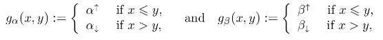
rewrite the equations of Question

(b) into a single equation in case \(S_{t}=\alpha S_{t-1}\), and a single equation in case \(S_{t}=\beta S_{t-1}\).

d) From the result of Question (c), derive an equation satisfied by \(\xi_{t}\left(S_{t-1}ight)\), and show that it admits a unique solution \(\xi_{t}\left(S_{t-1}ight)\).
Hint: Show that the piecewise affine function \[
\begin{aligned}
x \mapsto & f\left(x, S_{t-1}ight):=g_{\beta}\left(x, \xi_{t+1}\left(\beta S_{t-1}ight)ight)\left(x-\xi_{t+1}\left(\beta S_{t-1}ight)ight) \\
& -g_{\alpha}\left(x, \xi_{t+1}\left(\alpha S_{t-1}ight)ight)\left(x-\xi_{t+1}\left(\alpha S_{t-1}ight)ight)-ho \frac{\eta_{t+1}\left(\beta S_{t-1}ight)-\eta_{t+1}\left(\alpha S_{t-1}ight)}{\widetilde{S}_{t-1}}
\end{aligned}
\]
is strictly increasing in \(x \in \mathbb{R}\).

e) Find the expressions of \(\xi_{t}\left(S_{t-1}ight)\) and \(\eta_{t}\left(S_{t-1}ight)\) by solving the \(2 \times 2\) system of equations of Question (c).
Hint: The expressions have to use the quantities \[
g_{\alpha}\left(\xi_{t}\left(S_{t-1}ight), \xi_{t+1}\left(\alpha S_{t-1}ight)ight), \quad g_{\beta}\left(\xi_{t}\left(S_{t-1}ight), \xi_{t+1}\left(\beta S_{t-1}ight)ight)
\]
and they should be consistent with Proposition 3.12 when \(\lambda=0\), i.e. when \(\alpha^{\uparrow}=\alpha_{\downarrow}=\) \(1+a\) and \(\beta^{\uparrow}=\beta_{\downarrow}=1+b\), with \(ho=1+r\).

f) Find the value of \(g_{\alpha}\left(\xi_{t}\left(S_{t-1}ight), \xi_{t+1}\left(\alpha S_{t-1}ight)ight)\) in the following two cases:
i) \(f\left(\xi_{t+1}\left(\alpha S_{t-1}ight), S_{t-1}ight) \geqslant 0\), ii) \(f\left(\xi_{t+1}\left(\alpha S_{t-1}ight), S_{t-1}ight)i) \(f\left(\xi_{t+1}\left(\beta S_{t-1}ight), S_{t-1}ight) \geqslant 0\), ii) \(f\left(\xi_{t+1}\left(\beta S_{t-1}ight), S_{t-1}ight)

g) Hedge and price the call option with strike price \(K=\$ 2\) and \(N=2\) when \(S_{0}=8\), \(ho=1, \alpha=0.5, \beta=2\), and the transaction cost rate is \(\lambda=12.5 \%\). Provide sufficient details of hand calculations.
Remark: The evaluation of the terminal payoff uses the value of \(S_{2}\) only and is not affected by bid/ask prices.

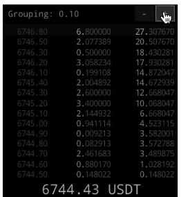
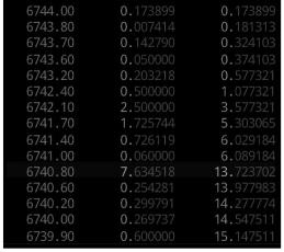
Figure 3.14: BTC/USD order book example.

In the above figure, ask prices are marked in red and bid prices are marked in green. The center column gives the quantity of the asset available at that row's bid or ask price, and the right column represents the cumulative volume of orders from the last-traded price until the current bid/ask price level. The large number in the center shows the last-traded price.

Transcribed Image Text:

t = 1,..., N, with 0 < a < 8. So < St = S = 380 Si = a So BSt-1 aSt-1 S = 8 So S2 = a8S0 S = So. Figure 3.12: Tree of market prices with N = 2.