In Example 16.15, we considered a count data model for the number of doctor visits by an individual as a function of a few explanatory variables. In this exercise, we expand the analysis using a larger data set in the data file, rwm 88 , and more explanatory variables. Adjust the data in the following ways: (i) omit individuals for whom \(H H N I N C 2=0\); (ii) create the variable \(L I N C=\ln (H H N I N C 2)\); (iii) create \(A G E 2=A G E^{2}\); (iv) create the variable \(P O S T=1\) (a postsecondary degree indicator variable) if \(F A C H H S=1\) or if \(U N I V=1\), and \(P O S T=0\) otherwise.

a. Using the first 3000 observations estimate a Poisson model explaining DOCVIS as a function of FEMALE, AGE, AGE2, SELF, LINC, POST, and PUBLIC. Discuss the signs and the significance of the coefficients on FEMALE, SELF, POST, and PUBLIC. Calculate the percentage increase in the expected number of doctor visits for each factor represented by these indicator variables.

b. Compute the estimated percentage change in the expected number of doctor visits associated with another year of age for a person who is 30 years old; who is 50 years old; and who is 70 years old.

c. Interpret the estimated coefficient of LINC.

d. Calculate the expected number of doctor visits for each person, EDOCVIS, and round this value to the nearest integer to obtain NVISITS, the predicted number of visits for each person. Create a variable that indicates a successful prediction. Let SUCCESS \(=1\) if NVISITS \(=\) DOCVIS and \(S U C C E S S=0\) otherwise. What is the percentage of successful predictions for observations \(1-3000\) ? What is the percentage of successful predictions for the remaining 979 observations?

e. Create SUCCESS1 which indicates a successful prediction of more than one doctor visit. That is, create a variable DOCVIS1 = 1 if an individual has more than one doctor visit, and PREDICT1 \(=1\) if the model has predicted more than one doctor visit. Let \(S U C C E S S 1=1\) if DOCVIS1 \(=\) PREDICT1 and SUCCESS1 \(=0\) otherwise. What is the percentage of successful predictions of more than one doctor visit for observations 1-3000? What is the percentage of successful predictions of more than one doctor visit for the remaining 979 observations?

Data From Example 16.15:-

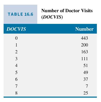
The economic analysis of the health care system is a vital area of research and public interest. In this example, we consider data used by Riphahn, Wambach, and Million (2003). \({ }^{22}\) The data file rwm88_small contains data on 1,200 individuals' number of doctor visits in the past three months (DOCVIS), their age in years ( \(A G E\) ), their sex (FEMALE), and whether or not they had public insurance (PUBLIC). The frequencies of doctor visits are illustrated in Table 16.6, with \(90.5 \%\) of the sample having eight or fewer visits.

Applying maximum likelihood estimation, we obtain the fitted model

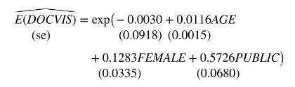
What can we say about these results? First, the coefficient estimates are all positive, implying that older individuals, females and those with public health insurance will have more doctor visits. Second, the coefficients of \(A G E\), FEMALE and PUBLIC are significantly different from zero, with \(p\)-values less than 0.01 . Using the fitted model, we can estimate the expected number of doctor visits. For example, the first person in the sample is a 29-year-old female who has public insurance. Substituting these values we estimate her expected number of doctor visits to be 2.816 , or 3.0 rounded to the nearest integer. Her actual number of doctor visits was zero.
Using the notion of generalized- \(R^{2}\), we can get a notion of how well the model fits the data by computing the squared correlation between DOCVIS and the predicted number of visits. If we use the rounded values, for example, 3.0 instead of 3.33 , the correlation is 0.1179 giving \(R_{g}^{2}=(0.1179)^{2}=0.0139\). The fit for this simple model is not very good as we might well expect. This model does not account for so many important factors, such as income, general health status, and so on. Different software packages report many different values, sometimes called pseudo- \(R^{2}\),  
with different meanings as well. We urge you to ignore all these values, including \(R_{g}^{2}\).
Instead of an \(R^{2}\)-like number, it is a good idea to report a test of overall model significance, analogous to the overall \(F\)-test for the regression model. The null hypothesis is that all the model coefficients, except the intercept, are equal to zero. We recommend the likelihood ratio statistic. See Section 16.2.7 for a discussion of this test in the context of the probit model. The test statistic is \(L R=2\left(\ln L_{U}-\ln L_{R}\right)\) where \(\ln L_{U}\) is the value of the \(\log\)-likelihood function for the full and unrestricted model and \(\ln L_{R}\) is the value of the log-likelihood function for the restricted model that assumes that the hypothesis is true. The restricted model in this case is \(E(D O C V I S)=\exp \left(\gamma_{1}\right)\). If the null hypothesis is true, the \(L R\) test statistic has a \(\chi_{(3)}^{2}\)-distribution in large samples. In our example, \(L R=174.93\) and the 0.95 percentile of the \(\chi_{(3)}^{2}\)-distribution is 7.815 . We reject the null hypothesis at the \(5 \%\) level of significance, and we conclude that at least one variable makes a significant impact on the number of doctor visits.
What about the magnitudes of the effects of these variables on the number of doctor visits? Treating \(A G E\) as continuous we can use (16.29) to compute a marginal effect,

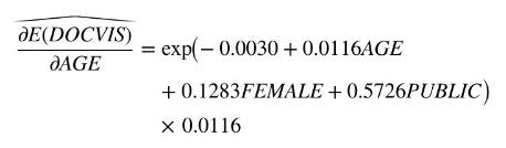
To evaluate this effect, we must insert values for \(A G E\), FEMALE, and PUBLIC. Let FEMALE \(=1\) and PUBLIC \(=1\).

If \(A G E=30\), the estimate is 0.0332 , with the \(95 \%\) interval estimate being [0.0261, 0.0402]. That is, we estimate for a 30 -year-old female with public insurance an additional year of age will increase her expected number of doctor visits in a 3-month period by 0.0332 . Because the marginal effect is a nonlinear function of the estimated parameters, the interval estimate uses a standard error calculated using the delta method. For \(A G E=70\), it is \(0.0528[0.0355,0.0702]\). The effect of another year of age is greater for older individuals, as you would expect.
Both FEMALE and PUBLIC are indicator variables, taking values zero and one. For these variables, we cannot evaluate the "marginal effect" using a derivative. Instead, we estimate the difference between the expected number of doctor visits for the two cases. For example,

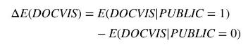
The calculated value of the difference is

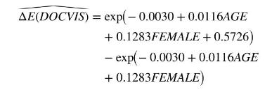
We estimate the difference for a 30 -year-old female to be 1.24 \([1.00,1.48]\), and for a 70 -year-old female, it is 1.98 [1.59, 2.36]. Women with public insurance visit the doctor significantly more than women of the same age who do not have public insurance.

Data From Equation 16.29:-

Transcribed Image Text:

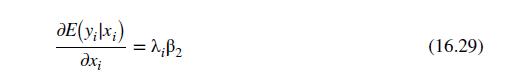
TABLE 16.6 Number of Doctor Visits (DOCVIS) T0 1234 DOCVIS 0 Number 443 1 200 163 111 51 5 49 6 37 7 7 8 25