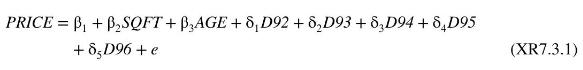
One of the key problems regarding housing prices in a region concerns construction of "price indexes." That is, holding other factors constant, have prices increased, decreased or stayed relatively constant in a particular area? As an illustration, consider a regression model for house prices (in \(\$ 1000\) s) on home sales from 1991 to 1996 in Stockton, CA, including as explanatory variables the size of the house (SQFT, in 100s of square feet), the age of the house (AGE) and annual indicator variables, such as \(D 92=1\) if the year is 1992 and 0 otherwise.

An alternative model employs a "trend" variable \(Y E A R=0,1, \ldots, 5\) for the years 1991-1996.

a. What is the expected selling price of a 10-year-old house with 2000 square feet of living space in each of the years 1991-1996 using equation (XR7.3.1)?

b. What is the expected selling price of a 10-year-old house with 2000 square feet of living space in each of the years 1991-1996 using equation (XR7.3.2)?

c. In order to choose between the models in (XR7.3.1) and (XR7.3.2), we propose a hypothesis test. What set of parameter constraints, or restrictions, would result in equation (XR7.3.1) equaling (XR7.3.2)? The sum of squared residuals from (XR7.3.1) is 2385745 and from (XR7.3.2) is 2387476. What is the test statistic for testing the restrictions that would make the two models equivalent? What is the distribution of the test statistic if the null hypotheses are true? What is the rejection region for a test at the \(5 \%\) level? If the sample size is \(N=4682\), what do you conclude?

d. Using the model in (XR7.3.1) the estimated coefficients of the indicator variables for 1992 and 1994, and their standard errors, are -4.393 (1.271) and -13.174 (1.211), respectively. The estimated covariance between these two coefficient estimators is 0.87825 . Test the null hypothesis that \(\delta_{3}=3 \delta_{1}\) against the alternative that \(\delta_{3} eq 3 \delta_{1}\) if \(N=4682\), at the \(5 \%\) level.

e. The estimated value of \(\tau\) in equation (XR7.3.2) is -4.12 . What is the estimated difference in the expected house price for a 10-year-old house with 2000 square feet of living space in 1992 and 1994. Using information in (d), how does this compare to the result using (XR7.3.1)?

Transcribed Image Text:

PRICE = B + BSQFT + AGE +8,D92 + 82D93 + 83D94 +8D95 +8D96 + e (XR7.3.1)