This exercise examines a supply and demand model for edible chicken, which the U.S. Department of Agriculture calls "broilers." The data for this exercise are in the file newbroiler, which is adapted from the data provided by Epple and McCallum (2006). We considered the demand equation in Exercise 11.20. It is

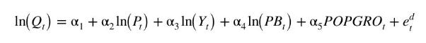
where \(Q\) is the per capita consumption of chicken, in pounds; \(Y\) is real per capita income; \(P\) is real price of chicken; \(P B\) is real price of beef, and \(P O P G R O\) is rate of population growth. What are the endogenous variables? What are the exogenous variables? The demand equation suffers from serial correlation. In the AR(1) model \(e_{t}^{d}=ho e_{t-1}^{d}+v_{t}^{d}\) the value of \(ho\) is large. Epple and McCallum estimate the model in "first difference" form:

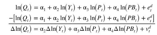
a. Regarding this specification (i) what changes do you notice after this transformation? (ii) Are the parameters of interest affected? (iii) If \(ho=1\), have we solved the serial correlation problem? (iv) What is the interpretation of the " \(\Delta\) " variables like \(\Delta \ln \left(Q_{t}\right)\) ? (v) What is the interpretation of the parameter \(\alpha_{2}\) ? (vi) What signs do you expect for each of the coefficients? Explain.

b. Using data from 1960 to 1999 , estimate the reduced-form, first-stage, equation for \(\Delta \ln \left(P_{t}\right)\) using instruments \(\ln \left(P F_{t}\right), T I M E_{t}, \ln \left(Q P R O D_{t-1}\right)\), and \(\ln \left(E X P T S_{t-1}\right)\). Can we conclude that at least one instrument is strong?

c. Estimate the first-stage equation for \(\Delta \ln \left(P_{t}\right)\) using instruments \(\Delta \ln \left(P F_{t}\right), \Delta \ln \left(Q P R O D_{t-1}\right)\), and \(\Delta \ln \left(E X P T S_{t-1}\right)\). Can we conclude that at least one instrument is strong? On logical grounds, why might we prefer these instruments to those in (b)?

d. Estimate the first-stage equation for \(\Delta \ln \left(P_{t}\right)\) using instrument \(\Delta \ln \left(P F_{t}\right)\). Can we conclude that the one instrument is strong?

e. Obtain the 2SLS estimates of the first-differenced demand equation using \(\Delta \ln \left(P F_{t}\right)\) as the instrument. In this estimation omit the constant term.

f. Obtain the 2SLS estimates of the first-differenced demand equation using \(\Delta \ln \left(P F_{t}\right)\) as the instrument including a constant term.

g. Compare the estimates of the key demand parameters in parts (e) and (f). Are the signs consistent with expectations? What are the interpretations of the estimated coefficients? Should an intercept be included in the differenced demand equation? Explain.

h. Construct a correlogram for the 2SLS residuals in part (e). Is there any evidence of serial correlation?

Data From Exercise 11.20:-

This exercise examines a supply and demand model for edible chicken, which the U.S. Department of Agriculture calls "broilers." The data for this exercise are in the file newbroiler, which is adapted from the data provided by Epple and McCallum (2006). We consider the demand equation in this exercise and the supply equation in Exercise 11.21.

a. Consider the demand equation:

where \(Q=\) per capita consumption of chicken, in pounds; \(Y=\) real per capita income; \(P=\) real price of chicken; \(P B=\) real price of beef; and \(P O P G R O=\) rate of population growth. What are the endogenous variables? What are the exogenous variables?

b. Using data from 1960 to 1999 , estimate the demand equation by OLS. Comment on the signs and significance of the estimates.

c. Test the OLS residuals from part (b) for serial correlation by constructing a correlogram and carrying out the \(T \times R^{2}\) test. What do you conclude about the presence of serial correlation?

d. Estimate the demand equation by 2SLS using as instruments \(\ln \left(P F_{t}\right), T I M E_{t}=Y E A R_{t}-1949\), \(\ln \left(Q P R O D_{t-1}\right)\), and \(\ln \left(E X P T S_{t-1}\right)\). Compare and contrast these estimates to the OLS estimates in part (a).

e. Estimate the reduced-form, first-stage, equation and test the joint significance of \(\ln \left(P F_{t}\right), T I M E_{t}\), \(\ln \left(Q P R O D_{t-1}\right)\), and \(\ln \left(E X P T S_{t-1}\right)\). Can we conclude that at least one instrument is strong?

f. Test the reduced-form equation for serial correlation using the \(T \times R^{2}\) test.

g. Estimate the reduced-form, first-stage, equation using HAC standard errors and test the joint significance of \(\ln \left(P F_{t}\right), T I M E_{t}, \ln \left(\right.\) QPROD \(\left._{t-1}\right)\), and \(\ln \left(E X P T S_{t-1}\right)\).

h. Obtain the 2SLS residuals from part (d). Construct a correlogram. Is there evidence of serial correlation? Obtain 2SLS estimates with HAC standard errors and compare the results to those in (d).

i. Test the validity of the surplus instruments using the Sargan test, discussed in Section 10.4.3, and the 2SLS estimates in part (d).

This exercise examines a supply and demand model for edible chicken, which the U.S. Department of Agriculture calls "broilers." The data for this exercise are in the file newbroiler, which is adapted from the data provided by Epple and McCallum (2006). We considered the demand equation in Exercise 11.20. The supply equation is

where \(Q P R O D\) is the aggregate production of young chickens, \(P F\) is nominal price index of broiler feed, and TIME = time index with \(1950=1, \ldots, 2001=52\). This supply equation is dynamic, with lagged production on the right-hand side. This predetermined variable is exogenous. TIME is included to capture technical progress in production.

a. What are the endogenous variables? What are the exogenous variables? What is the interpretation of the parameter \(\beta_{2}\) ? What signs do you expect for each of the parameters?

b. Using data from 1960 to 1999 , estimate the supply equation by OLS. Comment on the signs and significance of the estimates. Test the residuals for serial correlation. Is serial correlation present?

c. Estimate the reduced-form, first-stage, regression by OLS using the IVs \(\ln \left(Y_{t}\right), \ln \left(P B_{t}\right), P O P G R O\), and \(\ln \left(E X P T S_{t-1}\right)\). Test the joint significance of these variables. Can we conclude that we have at least one strong instrument?

d. Estimate the supply equation by 2SLS using the instruments listed in part (c). Compare and contrast these results to those in part (b).

e. Test the validity of the surplus instruments using the Sargan test, discussed in Section 10.4.3.

Transcribed Image Text:

In(Q), +ln(P) + 3 ln(Y,) + ln(PB) + , POPGRO, + + ed