We have defined the simple linear regression model to be \(y=\beta_{1}+\beta_{2} x+e\). Suppose, however, that we knew, for a fact, that \(\beta_{1}=0\).

a. What does the linear regression model look like, algebraically, if \(\beta_{1}=0\) ?

b. What does the linear regression model look like, graphically, if \(\beta_{1}=0\) ?

c. If \(\beta_{1}=0\), the least squares "sum of squares" function becomes \(S\left(\beta_{2}\right)=\sum_{i=1}^{N}\left(y_{i}-\beta_{2} x_{i}\right)^{2}\). Using the data in Table 2.4 from Exercise 2.3, plot the value of the sum of squares function for enough values of \(\beta_{2}\) for you to locate the approximate minimum. What is the significance of the value of \(\beta_{2}\) that minimizes \(S\left(\beta_{2}\right)\) ? Your computations will be simplified if you algebraically expand \(S\left(\beta_{2}\right)=\sum_{i=1}^{N}\left(y_{i}-\beta_{2} x_{i}\right)^{2}\) by squaring the term in parentheses and carrying through the summation operator.

d. Using calculus, show that the formula for the least squares estimate of \(\beta_{2}\) in this model is \(b_{2}=\) \(\sum x_{i} y_{i} / \sum x_{i}^{2}\). Use this result to compute \(b_{2}\) and compare this value with the value you obtained geometrically.

e. Using the estimate obtained with the formula in (d), plot the fitted (estimated) regression function. On the graph locate the point \((\bar{x}, \bar{y})\). What do you observe?

f. Using the estimate obtained with the formula in (d), obtain the least squares residuals, \(\hat{e}_{i}=y_{i}-b_{2} x_{i}\). Find their sum.

g. Calculate \(\sum x_{i} \hat{e}_{i}\).

Data From Table 2.4:-

Transcribed Image Text:

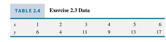
TABLE 2.4 Exercise 2.3 Data x y 1 6 24 3 11 49 69 17 53 13