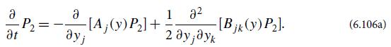
Consider a classical simple harmonic oscillator (e.g., the nanomechanical oscillator, LIGO mass on an optical spring, L-C-R circuit, or optical resonator briefly discussed in Ex. 6.17). Let the oscillator be coupled weakly to a dissipative heat bath with temperature T . The Langevin equation for the oscillator’s generalized coordinate x is Eq. (6.79). The oscillator’s coordinate x(t) and momentum p(t) ≡ mẋ together form a 2-dimensional Gaussian-Markov process and thus obey the 2-dimensional Fokker- Planck equation (6.106a). As an aid to solving this Fokker-Planck equation, change variables from {x, p} to the real and imaginary parts X₁ and X₂ of the oscillator’s complex amplitude:

Then {X₁, X₂} is a Gaussian-Markov process that evolves on a timescale ∼τr .

(a) Show that X₁ and X₂ obey the Langevin equation

(b) To compute the functions A_j(X) and B_jk(X) that appear in the Fokker-Planck equation (6.106a), choose the timescale △t to be short compared to the oscillator’s damping time τ_r but long compared to its period 2π/ω. By multiplying the Langevin equation successively by sin ωt and cos ωt and integrating from t = 0 to t = △t, derive equations for the changes △X₁ and △X₂ produced during △t by the fluctuating force F'(t) and its associated dissipation. [Neglect fractional corrections of order 1/(ω△t) and of order △t/τ_r]. Your equations should be analogous to Eq. (6.103a).

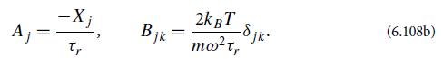
(c) By the same technique as was used in Ex. 6.22, obtain from the equations derived in part (b) the following forms of the Fokker-Planck functions:

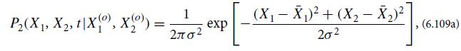
(d) Show that the Fokker-Planck equation, obtained by inserting functions (6.108b) into Eq. (6.106a), has the following Gaussian solution:

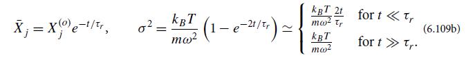
where the means and variance of the distribution are

(e) Discuss the physical meaning of the conditional probability (6.109a). Discuss its implications for the physics experiment described in Ex. 6.17, when the signal force acts for a time short compared to τ_r rather than long.

Equations

Data from Exercises 6.17

To measure a very weak sinusoidal force, let the force act on a simple harmonic oscillator with eigenfrequency at or near the force’s frequency, and measure the oscillator’s response. Examples range in physical scale from nanomechanical oscillators (∼1μm in size) with eigenfrequency ∼1GHz that might play a role in future quantum information technology (e.g., Chan et al., 2011), to the fundamental mode of a ∼10-kg sapphire crystal, to a∼40-kg LIGO mirror on which light pressure produces a restoring force, so its center of mass oscillates mechanically at frequency ∼100 Hz (e.g., Abbott et al., 2009a). The oscillator need not be mechanical; for example, it could be an L-C-R circuit, or a mode of an optical (Fabry-Perot) cavity.

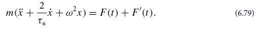
The displacement x(t) of any such oscillator is governed by the driven-harmonic oscillator equation

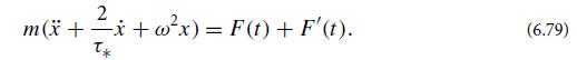
Herem,ω, and τ_∗ are respectively the effective mass, angular frequency, and amplitude damping time associated with the oscillator; F(t) is an external driving force; and F'(t) is the fluctuating force associated with the dissipation that gives rise to τ_∗. Assume that ωτ_∗>> 1 (weak damping).

Data from Exercises 6.22.

(a) Write down the explicit form of the Langevin equation for the x component of  velocity v(t) of a dust particle interacting with thermalized air molecules.

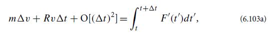
(b) Suppose that the dust particle has velocity v at time t. By integrating the Langevin  equation, show that its velocity at time t + Δt is v + Δv, where

with R the frictional resistance and m the particle’s mass. Take an ensemble  average of this and use F̅´ = 0 to conclude that the function A(v) appearing in  the Fokker-Planck equation (6.94) has the form

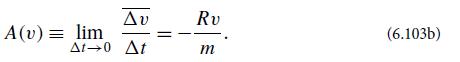
Compare this expression with the first of Eqs. (6.101) to conclude that the mean and relaxation time are v̅ = 0 and τ_r = m/R, respectively, in agreement with the second of Eqs. (6.53a) in the limit τ →∞and with Eq. (6.78).

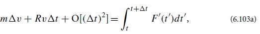
(c) From Eq. (6.103a) show that

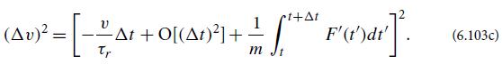
Take an ensemble average of this expression, and use

together with the Wiener-Khintchine theorem—to evaluate the terms involving F´ in terms of S_F´, which in turn is known from the fluctuation dissipation  theorem. Thereby obtain

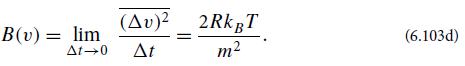
Combine with Eq. (6.101) and τ_r = m/R [from part (b)], to conclude that σ²_v  =  k_BT/m, in accord with the last of Eqs. (6.53a).

Transcribed Image Text:

(6.107) (1) (1)¹ X=[-(²x! + ¹x)] = x