In this exercise we will explore the welfare implications of the distributive pecuniary externalities discussed in section 11.1.3 in an international setting where countries are subject to "sudden stops" in their access to international financial markets.

Consider a model of three dates, \(t=0,1,2\) and two countries, Home and Foreign, each populated by a continuum of unit mass of identical agents. The two countries trade frictionlessly with each other. At every date, Home (Foreign) agents receive a constant endowment of \(Y\left(Y^{*}ight)\) units of the Home (Foreign) good. Agents in Home have log intertemporal preferences, and Home's consumption bundle is a Cobb-Douglas aggregate of the two goods:

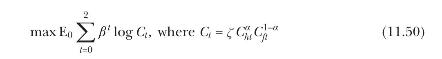
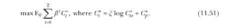
with \(\zeta \equiv \alpha^{-\alpha}(1-\alpha)^{-(1-\alpha)}\). Agents in Foreign have linear intertemporal preferences, and Foreign's consumption bundle is quasilinear in the Foreign good:

We assume throughout that we have an interior equilibrium, that is, \(C_{h t}, C_{f t}, C_{h t}^{*}, C_{f t}^{*}\), are strictly positive in all dates. By market clearing, \(Y=C_{h t}+C_{h t}^{*}\) and \(Y^{*}=C_{f t}+C_{f t}^{*}\) for all \(t\). Normalize the price of the foreign good in foreign currency to one, \(p_{f t}^{*} \equiv 1\). Then the terms of trade, generally defined as the ratio of export to import prices, are equal to the price of the home good in foreign currency, \(p_{h t}^{*}=p_{h t} / \varepsilon_{t}\), where \(\varepsilon_{t}\) denotes the nominal exchange rate (the price of foreign currency in units of domestic currency). Let \(p_{t}\) denote the consumption price index (CPI) of Home (in domestic currency), defined through \(p_{t} C_{t}=p_{h t} C_{h t}+\varepsilon_{t} C_{f t}\).
There exists a single asset, a one-period nominal bond in zero net supply paying in units of foreign currency with a nominal interest rate of \(1+i_{t+1}^{*}\). Home enters date 0 with a stock of debt \(D_{0}>0^{3}\) maturing at date 0 and optimally chooses the level of its debt maturing at date 1, \(D_{1}\). Given the finite-horizon setting, Home and Foreign are also subject to the terminal condition \(D_{3}=0\).
Home and Foreign are subject to the respective budget constraints (both expressed in units of foreign currency)

where \(T B_{t}=D_{t}-D_{t+1} /\left(1+i_{t+1}^{*}ight)\) is Home's trade balance.
Agents know that at date 1 a sudden stop will occur with some probability \(\pi, 0

(a) Derive the following intratemporal relationships expressing equilibrium quantities as functions of the terms of trade, \(p_{h t}^{*}\), and \(C_{t}\) that will be useful in the analysis to follow: \(p_{t} / \varepsilon_{t}=p_{h t}^{* \alpha}, C_{h t}=\alpha p_{h t}^{*-(1-\alpha)} C_{t}, C_{f t}=(1-\alpha) p_{h t}^{* \alpha} C_{t}, C_{h t}^{*}=\xi p_{h t}^{*-1}\), and \(C_{f t}^{*}=\) \(Y^{*}-(1-\alpha) p_{h t}^{* \alpha} C_{t}\).

(b) We assume that the financing constraint during the sudden stop only applies to Home agents. Therefore, the Euler equation of Foreign agents must hold at all dates and states. Show that \(1+i_{t+1}^{*}=1 / \beta\) for \(t=1,2\).

(c) Consider the case \(\pi=1\). We solve for the full equilibrium backward.
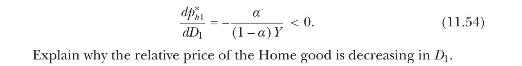
(i) Explain how a fall in the relative price of Home goods affects Home's date-1 consumption, \(C_{1}\), all else equal. Calculate the equilibrium terms of trade at date \(1, p_{h 1}^{*}\), as a function of \(D_{1}\) and the parameters of the model. Show that

(ii) Let \(V_{1}\left(D_{1}, p_{h 1}^{*}ight)\) and \(V_{1}^{*}\left(D_{1}, p_{h 1}^{*}ight)\) denote the date- 1 continuation value functions of Home and Foreign, respectively. Explain why the private (internalized) marginal cost for Home agents of higher debt maturing in the sudden-stop state is (the absolute value of) \(\partial V_{1} / \partial D_{1}\), while the social marginal cost for Home agents of higher debt is (the absolute value of) \(d V_{1} / d D_{1} \equiv \partial V_{1} / \partial D_{1}+\) \(\left(\partial V_{1} / \partial p_{h 1}^{*}ight)\left(d p_{h 1}^{*} / d D_{1}ight)\).
Show that

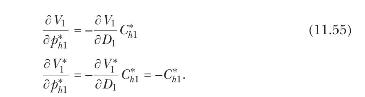
Why is the welfare impact of a change in the terms of trade proportional to \(C_{h 1}^{*}\) ?

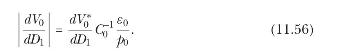
(iii) We now move to date 0 . Let \(V_{0}\left(D_{0}ight)\) and \(V_{0}^{*}\left(D_{0}ight)\) denote the ex-ante (date\(0)\) value functions of Home and Foreign, respectively. Show that, at the competitive equilibrium,

Use this result to argue that pecuniary externalities in this setting with \(\pi=1\) "net out" and the competitive equilibrium is constrained Pareto efficient. \({ }^{5}\)

(d) We now consider the case \(\pi

Denote the sudden-stop state (no-sudden-stop state) by \(s(n s)\). Once again, we solve backward.
(i) Consider Home's intertemporal consumption choice between dates 1 and 2 in the no-sudden-stop state. Show that \(D_{2}(n s)=D_{1} /(1+\beta), p_{h 1}^{*}(n s)=p_{h 2}^{*}(n s)\), and \(C_{1}(n s)=C_{2}(n s)\). Explain.
(ii) Show that \(d p_{h 1}^{*}(s) / d D_{1}=(1+\beta) d p_{h 1}^{*}(n s) / d D_{1}, p_{h 1}^{*}(s)(iii) Show that the condition

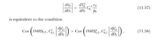
where \(I M R S_{0,1}\) and \(I M R S_{0,1}^{*}\) denote the intertemporal marginal rates of substitution between dates 0 and 1 of Home and Foreign agents, respectively, both in foreign currency units.
Argue that this inequality holds in the competitive equilibrium of the model, and hence the competitive equilibrium is constrained Pareto inefficient.

(e) Explain the intuition behind the different conclusions in parts

(c) and (d). How would the results be different in the \(\pi

Data from section 11.1.3

Transcribed Image Text:

max En Blog C, where G =CG 1-0 (11.50)