This exercise explores the properties of two recently proposed riskiness indices: the Aumann and Serrano (AS 2008)

Question:

This exercise explores the properties of two recently proposed riskiness indices: the Aumann and Serrano (AS 2008) index and the Foster and Hart (FH 2009) index.

A decision maker is characterized by an initial wealth level $W_{0}$ and von NeumannMorgenstern utility function $u$ over wealth with $u^{\prime}>0$ and $u^{\prime \prime}u\left(W_{0}ight)$. We only consider gambles with $\mathrm{E}[g]>0$ and $\operatorname{Pr}(g0$. For simplicity, we assume that gambles take finitely many values. Let $L_{g} \equiv \max (-g)$ and $M_{g} \equiv \max g$ denote the maximal loss and maximal gain of $g$, respectively.

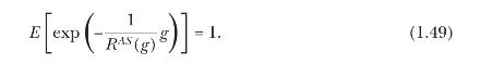
For any gamble $g$, the AS riskiness index $R^{A S}(g)$ is given by the unique positive solution to the equation

image text in transcribed

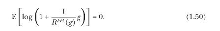
For any gamble $g$, the FH riskiness $R^{F H}(g)$ index is given by the unique positive solution to the equation

image text in transcribed

(a) Show that the AS riskiness index equals the level of risk tolerance that makes a CARA investor indifferent between accepting and rejecting the gamble. That is, an investor with CARA utility $u(w)=-\exp (-A w)$ will accept (reject) $g$ if \(A

(b) Show that the FH riskiness index equals the level of wealth that would make a log utility investor indifferent between accepting and rejecting the gamble. That is, a $\log$ investor with wealth $W_{0}>R^{F H}(g)\left(W_{0} \leq R^{F H}(g)ight)$ will accept (reject) $g$.

(c) Consider binary gambles with a loss of $L_{g}$ with probability $p_{L}$ and a gain $M_{g}$ with probability $1-p_{L}$. Calculate the values of the two indices for the binary gamble with $L_{g}=\$ 100, M_{g}=\$ 105$, and $p_{L}=1 / 2$ (Rabin 2000). Repeat for the binary gamble with $L_{g}=\$ 100, M_{g}=\$ 10,100$, and $p_{L}=1 / 2$. (The calculation is analytical for $\mathrm{FH}$ but numerical for AS.)

(d) Consider binary gambles with infinite gain, that is, $M_{g}$ arbitrarily large. Derive explicit formulas for the two indices as a function of $L_{g}$ and $p_{L}$ at the limit $M_{g} ightarrow+\infty$. Explain the intuition behind these formulas. Why do the indices assign nonzero riskiness to gambles with infinite expectation? What happens as $p_{L} ightarrow 0$ ?

(e) The Sharpe ratio, defined as the ratio of the mean of a gamble to its standard deviation, $S R(g) \equiv \mathrm{E}[g] / \sqrt{\operatorname{Var}(g)},{ }^{3}$ is a widely used measure of risk-adjusted portfolio returns. We can interpret its reciprocal as a riskiness index.
(i) Show by example that the (inverse) Sharpe ratio violates first-order stochastic dominance (and hence second-order stochastic dominance). That is, if gamble $h$ first-order stochastically dominates gamble $g$, then it is not always true that $S R(h) \geq S R(g)$.
(ii) AS (2008) propose a generalized version of the Sharpe ratio $\operatorname{GSR}(g) \equiv \mathrm{E}[g] /$ $R^{A S}(g)$, a measure of "riskiness-adjusted" expected returns. Argue that GSR respects second-order stochastic dominance (and hence first-order stochastic dominance).
(iii) Show that $\operatorname{GSR}(g)$ is ordinally equivalent to $S R(g)$ when $g$ is a normally distributed gamble.
Hint: use the probability density function of the normal distribution to show that $R^{A S}(g)=\operatorname{Var}(g) /(2 \mathrm{E}[g])$.