This problem asks you to use the GMM framework, presented in section 4.4, to analyze the two-beta asset pricing model of Campbell and Vuolteenaho (CV 2004). The data for this question can be found in an Excel spreadsheet on the textbook website, together with an accompanying explanatory document. \({ }^{13}\) The data include the excess return on the market together with the expected excess return and two components of the unexpected excess return, the news about cash flows \(N_{C F, t}\) and the news about discount rates \(-N_{D R, t}\). The news terms were estimated from a VAR as in CV. The data also include the riskless interest rate \(R_{f t}\) and the returns \(R_{i t}\) on a set of test assets, 9 of the 25 Fama-French portfolios sorted by size and book-to-market ratios.

We suggest using MATLAB or similar software that allows you to write flexible code. For all parts, document in detail the results and formulas from section 4.4 that you use in each step.

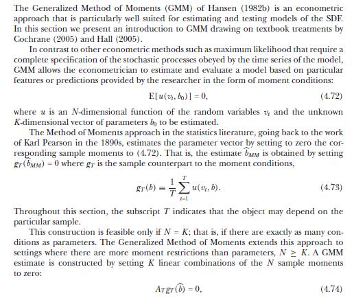
(a) Estimate the parameters of the linear stochastic discount factor model

Use 10 moment conditions (one for the risk-free asset and nine for the stock portfolios) of the form \(0=\mathrm{E}\left[M_{t}\left(1+R_{i t}ight)-1ight]\) and the identity weighting matrix \(W_{T}=\) \(I_{10}\).

(b) Estimate the long-run covariance matrix of the moments both under the null of the model that pricing errors are serially uncorrelated and by using the Newey-West HAC covariance matrix estimator. Estimate the covariance matrix of the parameter estimates under both estimates of the long-run covariance matrix. Do your results suggest pricing errors are serially correlated?
For the remaining parts, use the Newey-West estimator.

(c) For each parameter, report the \(t\)-statistic and \(p\)-value for the hypothesis that the parameter is zero.

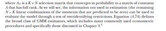
(d) Assume the following approximate and unconditional version of the first-order condition (9.40):

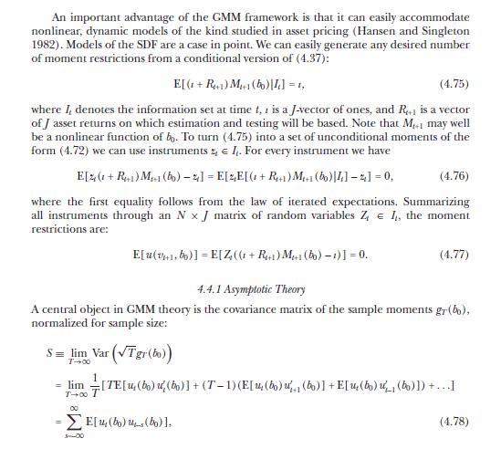
(i) What restriction does this condition impose on the parameters of SDF specification (9.74)?
(ii) Test this restriction using a Wald test. Is it rejected?
(iii) Provide an estimate of \(\gamma\) and the standard error of this estimate. Hint: Use the delta method.

(e) Return to the general model and compute the second-stage estimates of the parameters in (9.74). Repeat parts (c), (d) (ii), and (d) (iii) for the second-stage estimates. How do your answers differ?

Equation 9.74

(f) Finally, perform a \(\chi^{2}\)-test of overidentifying restrictions using the second-stage estimates. What is the \(p\)-value of the test? Comment on the empirical success of the model.

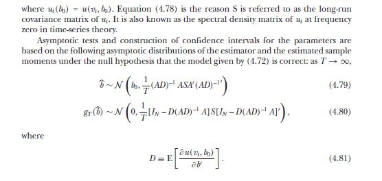
Data from section 4.4

Transcribed Image Text:

M = a + b(NDR) + CNCF,/- (9.74)