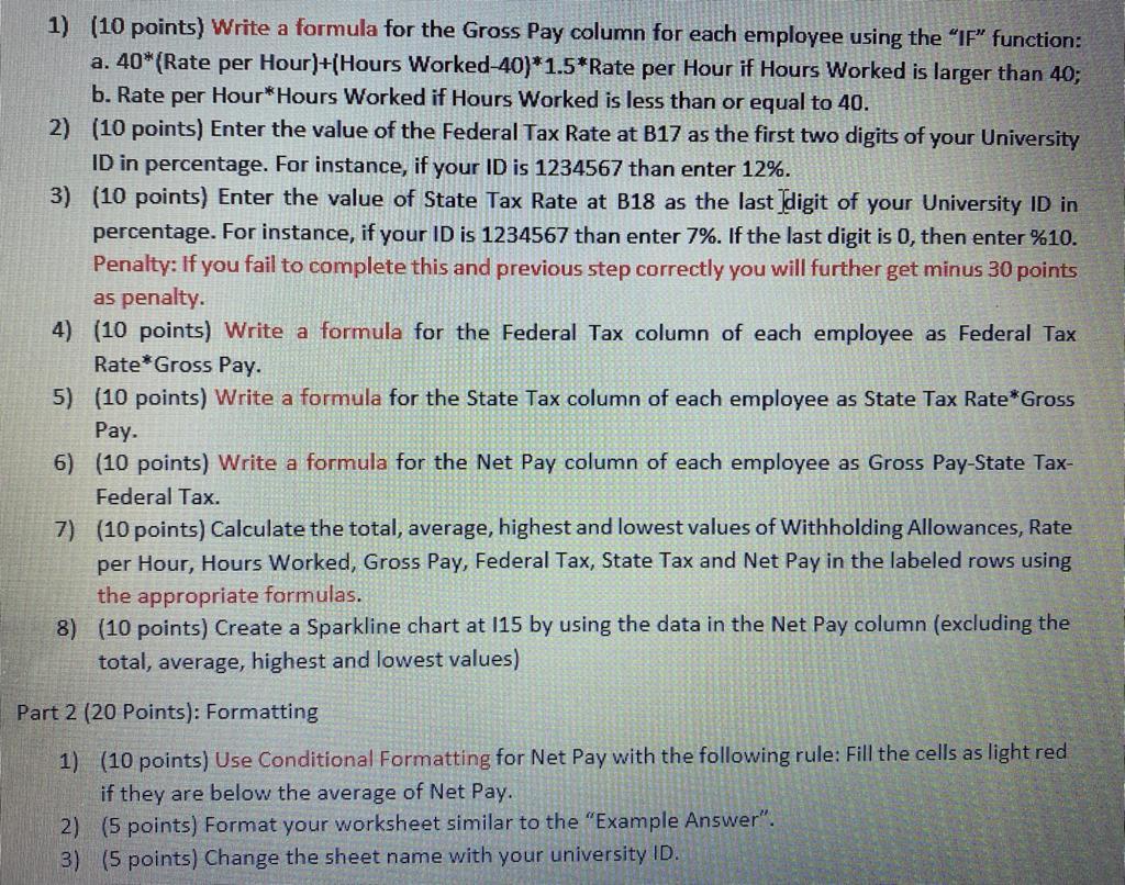
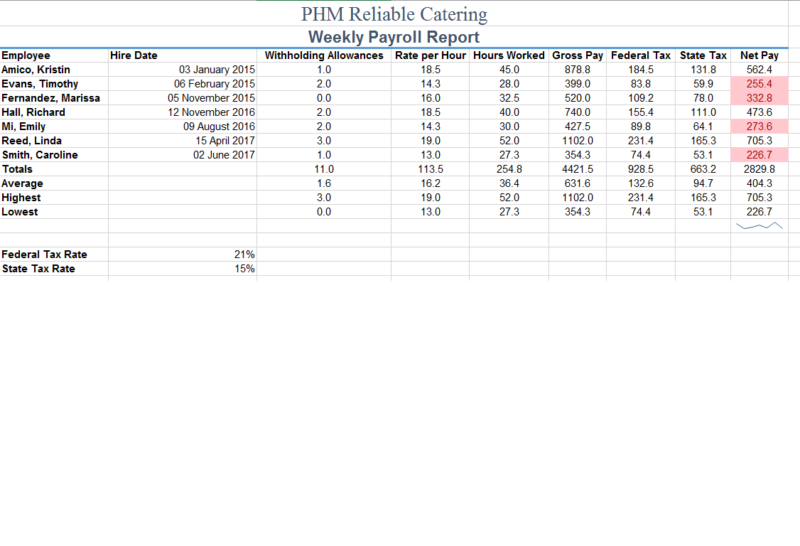
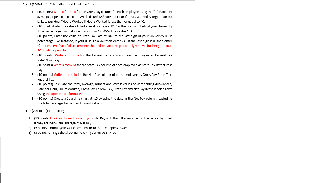
1) (10 points) Write a formula for the Gross Pay column for each employee using the "IF" function: a. 40*(Rate per Hour)+(Hours Worked-40)*1.5*Rate per Hour if Hours Worked is larger than 40; b. Rate per Hour*Hours Worked if Hours Worked is less than or equal to 40. 2) (10 points) Enter the value of the Federal Tax Rate at B17 as the first two digits of your University ID in percentage. For instance, if your ID is 1234567 than enter 12%. 3) (10 points) Enter the value of State Tax Rate at B18 as the last digit of your University ID in percentage. For instance, if your ID is 1234567 than enter 7%. If the last digit is 0, then enter %10. Penalty: If you fail to complete this and previous step correctly you will further get minus 30 points as penalty. 4) (10 points) Write a formula for the Federal Tax column of each employee as Federal Tax Rate Gross Pay. 5) (10 points) Write a formula for the State Tax column of each employee as State Tax Rate *Gross Pay. 6) (10 points) Write a formula for the Net Pay column of each employee as Gross Pay-State Tax- Federal Tax. 7) (10 points) Calculate the total, average, highest and lowest values of Withholding Allowances, Rate per Hour, Hours Worked, Gross Pay, Federal Tax, State Tax and Net Pay in the labeled rows using the appropriate formulas. 8) (10 points) Create a Sparkline chart at 115 by using the data in the Net Pay column (excluding the total, average, highest and lowest values) Part 2 (20 Points): Formatting 1) (10 points) Use Conditional Formatting for Net Pay with the following rule: Fill the cells as light red if they are below the average of Net Pay. 2) (5 points) Format your worksheet similar to the "Example Answer". 3) (5 points) Change the sheet name with your university ID. Hire Date Employee Amico, Kristin Evans, Timothy Fernandez, Marissa Hall, Richard Mi, Emily Reed, Linda Smith, Caroline Totals Average Highest Lowest 03 January 2015 06 February 2015 05 November 2015 12 November 2016 09 August 2016 15 April 2017 02 June 2017 PHM Reliable Catering Weekly Payroll Report Withholding Allowances Rate per Hour Hours Worked Gross Pay Federal Tax State Tax Net Pay 1.0 18.5 45.0 878.8 184.5 131.8 562.4 2.0 14.3 28.0 399.0 83.8 59.9 255.4 0.0 16.0 32.5 520.0 109.2 78.0 332.8 2.0 18.5 400 740.0 155.4 111.0 473.6 2.0 14.3 30.0 427.5 89.8 273.6 3.0 19.0 52.0 1102.0 231.4 165.3 705.3 1.0 13.0 27.3 354.3 74.4 53.1 226.7 11.0 113.5 254.8 4421.5 928.5 663.2 2829.8 1.6 16.2 36.4 631.6 132.6 404.3 3.0 19.0 52.0 1102.0 231.4 165.3 705.3 0.0 27.3 354.3 74.4 226.7 64.1 94.7 13.0 53.1 Federal Tax Rate State Tax Rate 21% 15% Part 1 (80 Points): Calculations and Sparkline Chart 1) (10 points) Write a formula for the Gross Pay column for each employee using the "IF" function: a. 40*(Rate per Hour)+(Hours Worked-40)*1.5*Rate per Hour if Hours Worked is larger than 40; b. Rate per Hour*Hours Worked if Hours Worked is less than or equal to 40. 2) (10 points) Enter the value of the Federal Tax Rate at B17 as the first two digits of your University ID in percentage. For instance, if your ID is 1234567 than enter 12%. 3) (10 points) Enter the value of State Tax Rate at B18 as the last digit of your University ID in percentage. For instance, if your ID is 1234567 than enter 7%. If the last digit is O, then enter %10. Penalty: If you fail to complete this and previous step correctly you will further get minus 30 points as penalty. 4) (10 points) Write a formula for the Federal Tax column of each employee as Federal Tax Rate"Gross Pay. 5) (10 points) Write a formula for the State Tax column of each employee as State Tax Rate*Gross Pay. 6) (10 points) Write a formula for the Net Pay column of each employee as Gross Pay-State Tax- Federal Tax. 7) (10 points) Calculate the total, average, highest and lowest values of Withholding Allowances, Rate per Hour, Hours Worked, Gross Pay, Federal Tax, State Tax and Net Pay in the labeled rows using the appropriate formulas. 8) (10 points) Create a Sparkline chart at 115 by using the data in the Net Pay column (excluding the total, average, highest and lowest values) Part 2 (20 Points): Formatting 1) (10 points) Use Conditional Formatting for Net Pay with the following rule: Fill the cells as light red if they are below the average of Net Pay. 2) (5 points) Format your worksheet similar to the "Example Answer". 3) (5 points) Change the sheet name with your university ID