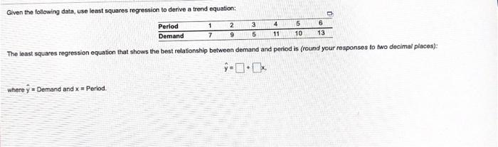
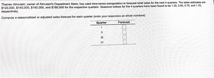
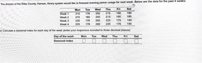
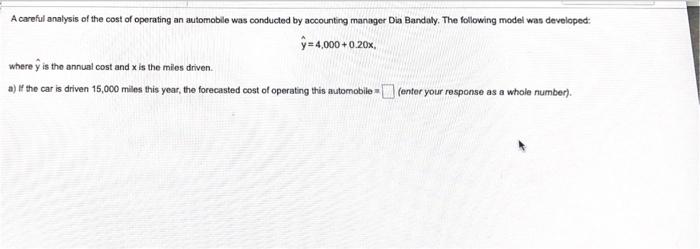
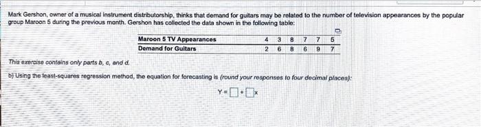
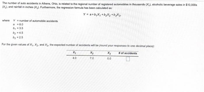
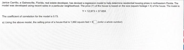
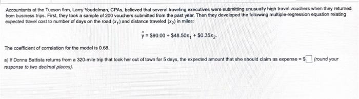
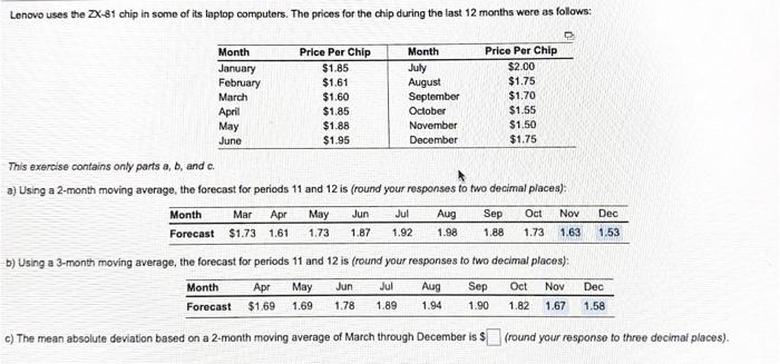
1 5 6 3 5 4 11 7 9 10 13 Given the following data, use least squares regression to derive a trend equation: Period 2 Demand The least squares regression equation that shows the best relationship between demand and period is (round your responses to two decimal places): 9-11 where y Demand and Period Thamer Almutairi, owner of Almutairi's Department Store, has used time series extrapolation to forecast retail sales for the next 4 quarters. The sales estimates are $120,000, $140,000, $160,000, and $180,000 for the respective quarters, Seasonal indices for the 4 quarters have been found to be 1.25, 0.90, 0.75, and 1.10. respectively Compute a seasonalized or adjusted sales forecast for each quarter (enter your responses as whole numbers). Quarter Forecast 1 H1 111 IV The director of the Riley County, Kansas, library system would like to forecast evening patron usage for next week. Below are the data for the past 4 weeks: Week 1 Week 2 Week 3 Week 4 Mon 210 215 220 225 Tue 178 180 176 178 Wed 250 250 260 260 Thu 215 213 220 225 Fri 160 165 175 176 Sat 180 185 190 190 4) Calculate a seasonal index for each day of the week (enter your responses rounded to three decimal places). Mon Tue Wed Thu Fri Sat Day of the week Seasonal index A careful analysis of the cost of operating an automobile was conducted by accounting manager Dia Bandaly. The following model was developed 9=4,000+0 20x, where y is the annual cost and is the miles driven a) if the car is driven 15,000 miles this year, the forecasted cost of operating this automobile - center your response as a whole number). 4 Mark Gershon, owner of a musical instrument distributorship, thinks that demand for guitars may be related to the number of television appearances by the popular group Maroon 5 during the previous month. Gershon has collected the data shown in the following table: Maroon 5 TV Appearances 3 8 7 7 5 Demand for Guitars 2 6 8 6 9 7 This exercise contains only parts b, c, and d. bj Using the teast-squares regression method, the equation for forecasting is (round your responses to four decimal places): Y-0.[ The number of auto accidents in Athens, Ohio, is related to the regional number of registered automobiles in thousands (X), alcoholic beverage sales in 510,000s X), and rainfall in inches (X). Furthermore, the regression formula has been calculated as: Y = a+byx, +b3X2 +by%3 where y = number of automobile accidents a = 8.0 by = 3.5 by = 4.5 Dy - 2.5 For the given values of X, X2, and X3, the expected number of accidents will be (round your responses to one decimal place): X X # of accidents X2 7.0 4.0 0.0 Janice Carrillo, a Gainesville, Florida, real estate developer, has devised a regression model to help determine residential housing prices in northeastern Florida. The model was developed using recent sales in a particular neighborhood. The price (Y) of the house is based on the size (square footage = X) of the house. The model is: Y = 12,973 + 37.65% The coefficient of correlation for the model is 0.73. 3) Using the above model, the selling price of a house that is 1,860 square feet = $contor a whole number). Accountants at the Tucson firm, Larry Youdelman, CPAs, believed that several traveling executives were submitting unusually high travel vouchers when they retumed from business trips. First, they took a sample of 200 vouchers submitted from the past year. Then they developed the following multiple-regression equation relating expected travel cost to number of days on the road (xs) and distance traveled (x2) in miles: = $90.00 + $48.50x, + $0.35x2 The coefficient of correlation for the model is 0.68. a) Donna Battista returns from a 320-mile trip that took her out of town for 5 days, the expected amount that she should claim as expense = $(round your response to two decimal places) Lenovo uses the ZX-81 chip in some of its taptop computers. The prices for the chip during the last 12 months were as follows: Month Price Per Chip Month Price Per Chip January $1.85 July $2.00 February $1.61 August $1.75 March $1.60 September $1.70 April $1.85 October $1.55 May $1.88 November $1.50 June $1.95 December $1.75 This exercise contains only parts a, b, and c. a) Using a 2-month moving average, the forecast for periods 11 and 12 is (round your responses to two decimal places): Month Mar Apr May Jun Aug Sep Oct Nov Forecast $1.73 1.61 1.73 1.92 1.98 1.88 1.73 1.63 Dec 1.87 1.53 b) Using a 3-month moving average, the forecast for periods 11 and 12 is (round your responses to two decimal places): Month May Jun Jul Aug Sep Oct Nov Forecast $1.69 1.69 1.78 1.89 1.94 1.90 1.82 1.67 Apr Dec 1.58 c) The mean absolute deviation based on a 2-month moving average of March through December is $ (round your response to three decimal places)