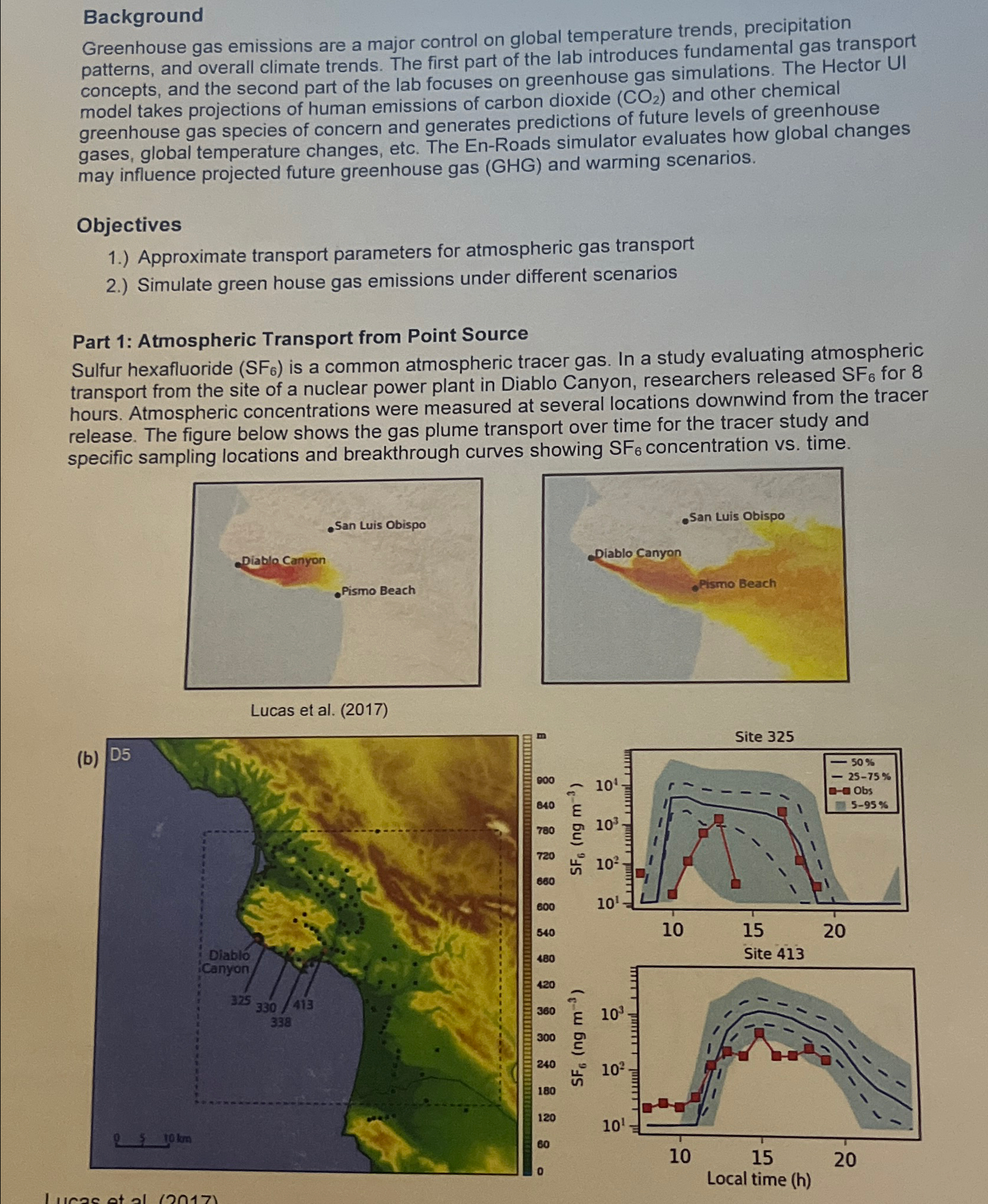
$1.)$ Approximate the possible range of average wind velocities based on the two $S{F}_6$ breakthrough curves at Site $325$ and Site $413.($Hint: Use the $50\%$ model curves for analysis, and state distances from source approximated from figure.$)$

$2.)$ Explain why $S{F}_6$ concentrations at Site $325$ are much higher than Site $413.$

$3.)$ If the flow rate from the smoke stack is $90\frac{m^3}{sec}$ of exhaust gases at a temperature of $70C.$ Outside air temperature is $25C,$ and wind speed is $4\frac{m}{sec}.$ The stack is $30m$ tall, with a diameter of $60cm.$ What is the plume height at the edge of the property $50m$ downwind?

$H=1\mathrm{.}6F_b^{\frac{1}{3}}\frac{x^{\frac{2}{3}}}{u}$

$F_b=g(\frac{d^{2}V}{4})(\frac{T_s-T_a}{T_s})$

$H=$ plume rise $L$

$F_b=$ buoyancy flux parameter $\frac{L^4}{T^3}$

$x=$ downwind distance $L,$

$u=$ wind speed $\frac{L}{T}$

$g=$ acceleration due to gravity $\frac{L}{T^2}$

$d=$ stack diameter $[$L$]$

$V=$ stack gas velocity $\frac{L}{T}$

$T_s=$ absolute stack gas temperature $(K)$

$T_a=$ absolute ambient air temperature $(K)$

Background

Greenhouse gas emissions are a major control on global temperature trends, precipitation patterns, and overall climate trends. The first part of the lab introduces fundamental gas transport concepts, and the second part of the lab focuses on greenhouse gas simulations. The Hector UI model takes projections of human emissions of carbon dioxide $(C{O}_2)$ and other chemical greenhouse gas species of concern and generates predictions of future levels of greenhouse gases, global temperature changes, etc. The En$-$Roads simulator evaluates how global changes may influence projected future greenhouse gas $($GHG$)$ and warming scenarios.

Objectives

$1.)$ Approximate transport parameters for atmospheric gas transport

$2.)$ Simulate green house gas emissions under different scenarios

Part $1$: Atmospheric Transport from Point Source

Sulfur hexafluoride $(S{F}_6)$ is a common atmospheric tracer gas. In a study evaluating atmospheric transport from the site of a nuclear power plant in Diablo Canyon, researchers released SF $S_6$ for $8$ hours. Atmospheric concentrations were measured at several locations downwind from the tracer release. The figure below shows the gas plume transport over time for the tracer study and specific sampling locations and breakthrough curves showing $S{F}_6$ concentration vs$.$ time.

$($b$)$