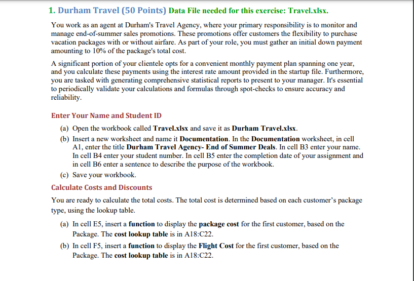
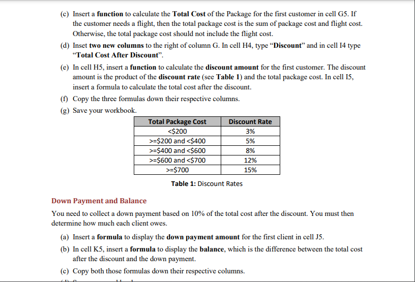
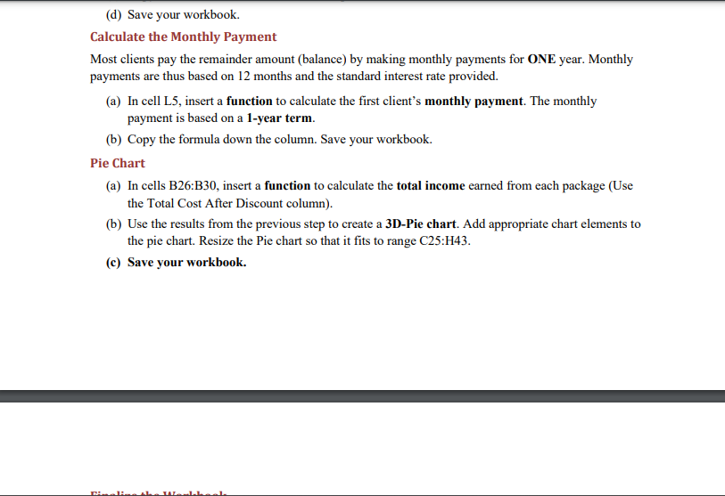
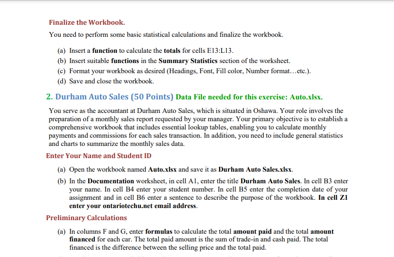
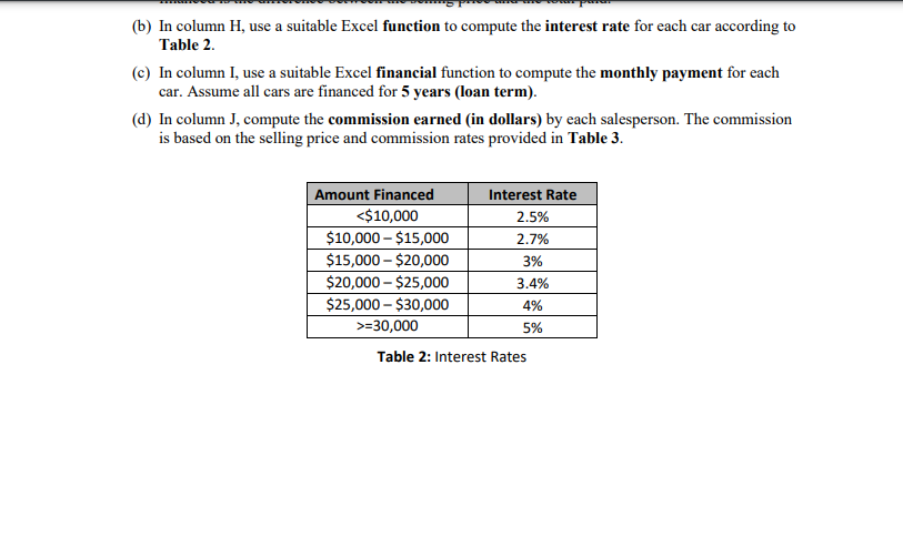
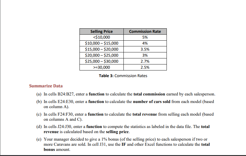
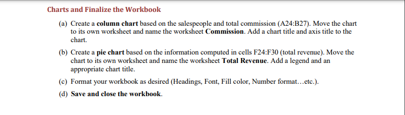
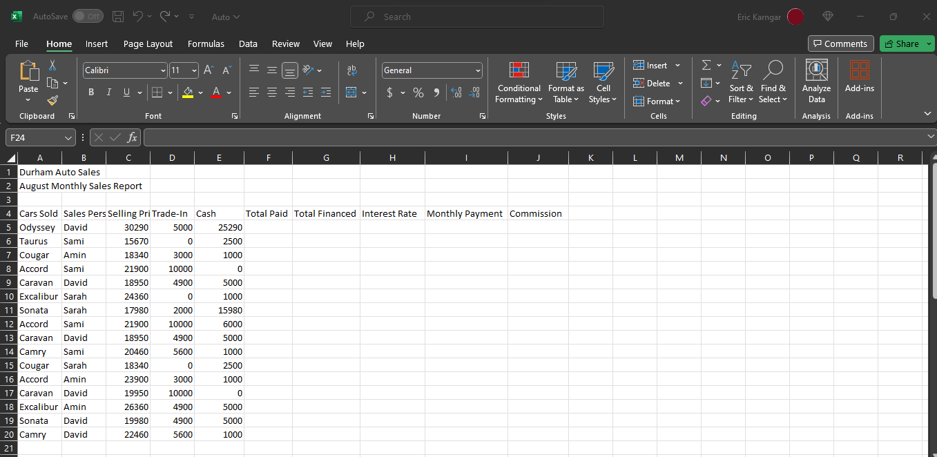
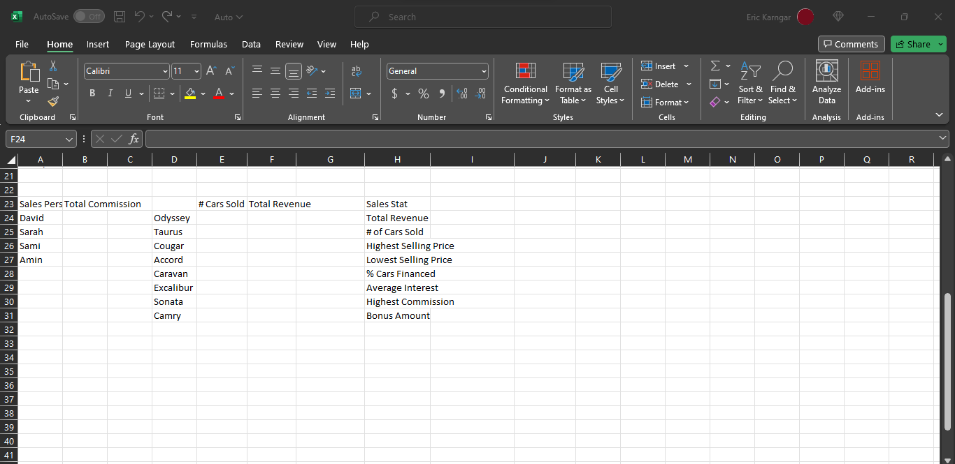
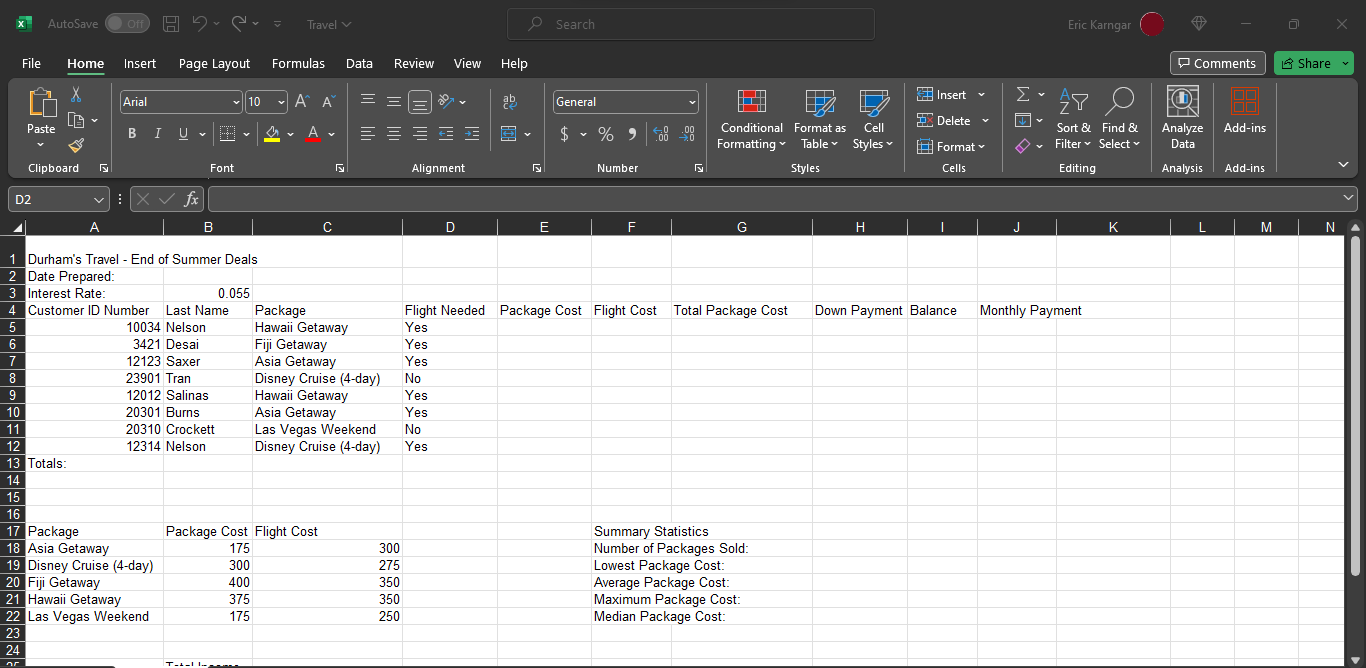
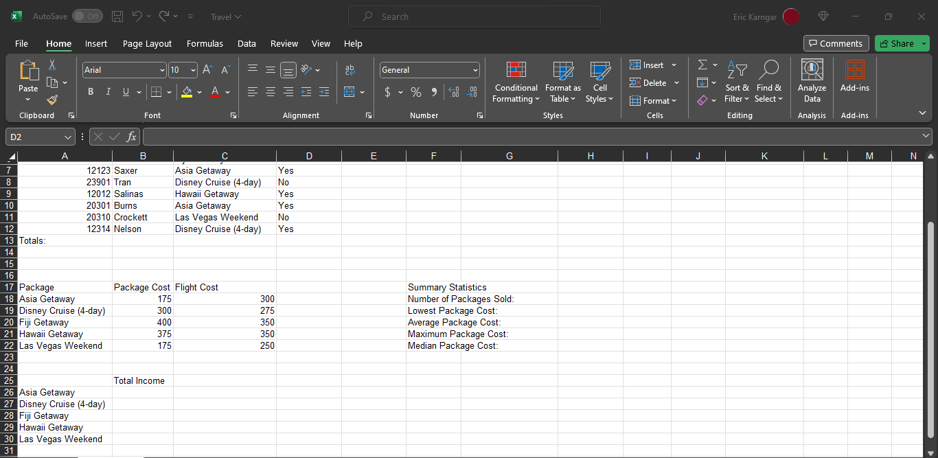
1. Durham Travel (50 Points) Data File needed for this exercise: Travel.xIsx. You work as an agent at Durham's Travel Agency, where your primary responsibility is to monitor and manage end-of-summer sales promotions. These promotions offer customers the flexibility to purchase vacation packages with or without airfare. As part of your role, you must gather an initial down payment amounting to 10% of the package's total cost. A significant portion of your clientele opts for a convenient monthly payment plan spanning one year, and you calculate these payments using the interest rate amount provided in the startup file. Furthermore, you are tasked with generating comprehensive statistical reports to present to your manager. It's essential to periodically validate your calculations and formulas through spot-checks to ensure accuracy and reliability. Enter Your Name and Student ID (a) Open the workbook called Travel.xIsx and save it as Durham Travel.xIsx. (b) Insert a new worksheet and name it Documentation. In the Documentation worksheet, in cell Al, enter the title Durham Travel Agency- End of Summer Deals. In cell B3 enter your name. In cell B4 enter your student number. In cell B5 enter the completion date of your assignment and in cell B6 enter a sentence to describe the purpose of the workbook. (c) Save your workbook. Calculate Costs and Discounts You are ready to calculate the total costs. The total cost is determined based on each customer's package type, using the lookup table. (a) In cell E5, insert a function to display the package cost for the first customer, based on the Package. The cost lookup table is in A18:C22. (b) In cell F5, insert a function to display the Flight Cost for the first customer, based on the Package. The cost lookup table is in A18:C22.(c) Insert a function to calculate the Total Cost of the Package for the first customer in cell G5. If the customer needs a flight, then the total package cost is the sum of package cost and flight cost. Otherwise, the total package cost should not include the flight cost. (d) Inset two new columns to the right of column G. In cell H4, type "Discount" and in cell 14 type "Total Cost After Discount". (e) In cell H5, insert a function to calculate the discount amount for the first customer. The discount amount is the product of the discount rate (see Table 1) and the total package cost. In cell 15, insert a formula to calculate the total cost after the discount. (f) Copy the three formulas down their respective columns. (g) Save your workbook. Total Package Cost Discount Rate =$200 and =$400 and =$600 and =$700 15% Table 1: Discount Rates Down Payment and Balance You need to collect a down payment based on 10% of the total cost after the discount. You must then determine how much each client owes. (a) Insert a formula to display the down payment amount for the first client in cell J5. (b) In cell K5, insert a formula to display the balance, which is the difference between the total cost after the discount and the down payment. (c) Copy both those formulas down their respective columns.{d} Save your workbook. Calculate the Monthly Payment Most clients pay the remainder amount {balance} by making monthly payments for ONE. year. Monthly payments are thus based on 12 months and the standard interest rate provided. {a} In cell L5, insert a funetion to calculate the rst client's monthly payment. The monthly payment is based on a 1-year term. {b} Copy the formula down the column. Save your workbook. Pie l[Shaft {a} In cells Bll. insert a function to calculate the total income earned from each package [Use the Total Cost After Discount column]. {b} Use the results from the previous step to create a ll-Pie chart. Add appropriate chart elements to the pie chart. Resize the Pie chart so that it ts to range C25:H43. {e} Save your workbook. Finalize the Workbook. You need to perform some basic statistical calculations and finalize the workbook. (a) Insert a function to calculate the totals for cells E13:L13. (b) Insert suitable functions in the Summary Statistics section of the worksheet. (c) Format your workbook as desired (Headings, Font, Fill color, Number format... etc.). (d) Save and close the workbook. 2. Durham Auto Sales (50 Points) Data File needed for this exercise: Auto.xIsx. You serve as the accountant at Durham Auto Sales, which is situated in Oshawa. Your role involves the preparation of a monthly sales report requested by your manager. Your primary objective is to establish a comprehensive workbook that includes essential lookup tables, enabling you to calculate monthly payments and commissions for each sales transaction. In addition, you need to include general statistics and charts to summarize the monthly sales data. Enter Your Name and Student ID (a) Open the workbook named Auto.xIsx and save it as Durham Auto Sales.xIsx. (b) In the Documentation worksheet, in cell Al, enter the title Durham Auto Sales. In cell B3 enter your name. In cell B4 enter your student number. In cell B5 enter the completion date of your assignment and in cell B6 enter a sentence to describe the purpose of the workbook. In cell ZI enter your ontariotechu.net email address. Preliminary Calculations (a) In columns F and G, enter formulas to calculate the total amount paid and the total amount financed for each car. The total paid amount is the sum of trade-in and cash paid. The total financed is the difference between the selling price and the total paid.(b) In column H, use a suitable Excel function to compute the interest rate for each car according to Table 2. (c) In column I, use a suitable Excel financial function to compute the monthly payment for each car. Assume all cars are financed for 5 years (loan term). (d) In column J, compute the commission earned (in dollars) by each salesperson. The commission is based on the selling price and commission rates provided in Table 3. Amount Financed Interest Rate =30,000 5% Table 2: Interest RatesSelling Price Commission Rate =30,000 2.5% Table 3: Commission Rates Summarize Data (a) In cells B24:B27, enter a function to calculate the total commission earned by each salesperson. (b) In cells E24:E30, enter a function to calculate the number of cars sold from each model (based on column A). (c) In cells F24:F30, enter a function to calculate the total revenue from selling each model (based on columns A and C). (d) In cells J24:J30, enter a function to compute the statistics as labeled in the data file. The total revenue is calculated based on the selling price. (e) Your manager decided to give a 1% bonus (of the selling price) to each salesperson if two or more Caravans are sold. In cell J31, use the IF and other Excel functions to calculate the total bonus amount.Charts and Finalize the Workbook (a) Create a column chart based on the salespeople and total com mission [A24:BE?]. Move the chart to its own worksheet and name the worksheet Commission. Add a chart title and axis title to the chart. {1:} Create a pie chart based on the information computed in cells F24:F3l] [total revenue}. Move the chart to its own worksheet and name the worksheet Total Raven no. Add a legend and an appropriate chart title. (c) Format your workbook as desired (Headings, Font1 Fill color1 Number tormat. . .etc.]. {d} Save and close the workbook. X AutoSave Off) Auto v Search Eric Karngar File Home Insert Page Layout Formulas Data Review View Help Comments Share X Insert Calibri 11 A A General AY O * Delete v Paste B I U $ v % 9 Conditional Format as Cell Sort & Find & Analyze Add-ins A = + = Formatting Table v Styles v [ Format Filter ~ Select Data Clipboard Font Alignment Number Styles Cells Editing Analysis Add-ins F24 X v fx B C D E F G H K M IN O P Q R Durham Auto Sales 2 August Monthly Sales Report 3 Cars Sold Sales Pers Selling Pri Trade-In Cash Total Paid Total Financed Interest Rate Monthly Payment Commission 5 Odyssey David 30290 5000 25290 6 Taurus Sami 15670 0 2500 Cougar Amin 18340 3000 1000 8 Accord Sami 21900 10000 9 Caravan David 18950 4900 5000 10 Excalibur Sarah 24360 1000 11 Sonata Sarah 17980 2000 15980 12 Accord Sami 21900 10000 6000 13 Caravan David 18950 4900 5000 14 Camry Sami 20460 5600 1000 15 Cougar Sarah 18340 2500 16 Accord Amin 23900 3000 1000 17 Caravan David 19950 10000 0 18 Excalibur Amin 26360 4900 5000 19 Sonata David 19980 4900 5000 20 Camry David 22460 5600 1000 21X AutoSave Off Auto v Search Eric Karngar X File Home Insert Page Layout Formulas Data Review View Help Comments Share X Insert Calibri 11 General AY O Delete Paste BIU $ % 9 Conditional Format as Cell Sort & Find & Analyze Add-ins Formatting * Table Styles ~ [ Format Filter * Select Data Clipboard Font Is Alignment Number Styles Cells Editing Analysis Add-ins F24 [XV fx B C D E F G H K M N O P Q R 21 22 23 Sales Pers Total Commission # Cars Sold Total Revenue Sales Stat 24 David Odyssey Total Revenue 25 Sarah Taurus # of Cars Sold 26 Sami Cougar Highest Selling Price 27 Amin Accord Lowest Selling Price 28 Caravan % Cars Financed 29 Excalibur Average Interest 30 Sonata Highest Commission 31 Camry Bonus Amount 32 33 34 35 36 37 38 39 40 41X AutoSave Off Travel v Search Eric Karngar X File Home Insert Page Layout Formulas Data Review View Help Comments Share X Insert Arial 10 General AY O D Paste % ? Conditional Format as Cell Delete I V Add-ins B I U + = Sort & Find & Analyze Formatting Table Styles ~ [ Format Filter * Select Data Clipboard Font Alignment Number Styles Cells Editing Analysis Add-ins D2 X v fx A B C D E F G H J K M N Durham's Travel - End of Summer Deals 2 Date Prepared: 3 Interest Rate: 0.055 4 Customer ID Number Last Name Package Flight Needed Package Cost Flight Cost Total Package Cost Down Payment Balance Monthly Payment 5 10034 Nelson Hawaii Getaway Yes 6 3421 Desai Fiji Getaway Yes 12123 Saxer Asia Getaway Yes 8 23901 Tran Disney Cruise (4-day) No 12012 Salinas Hawaii Getaway Yes 10 20301 Burns Asia Getaway Yes 11 20310 Crockett Las Vegas Weekend No 12 12314 Nelson Disney Cruise (4-day) Yes 13 Totals: 14 15 16 17 Package Package Cost Flight Cost Summary Statistics 18 Asia Getaway 175 300 Number of Packages Sold: 19 Disney Cruise (4-day) 300 275 Lowest Package Cost: 20 Fiji Getaway 400 350 Average Package Cost: 21 Hawaii Getaway 375 350 Maximum Package Cost: 22 Las Vegas Weekend 175 250 Median Package Cost: 23 24X X AutoSave Off Travel v Search Eric Karngar File Home Insert Page Layout Formulas Data Review View Help Comments Share X Insert Arial 10 General AY O Cell Delete I V Paste Sort & Find & Analyze Add-ins B I U $ ~ % 9 Conditional Format as Formatting ~ Table Styles v [ Format Filter * Select Data Clipboard Font Is Alignment Number Styles Cells Editing Analysis Add-ins D2 XV fx A B C D E F G H J K M N 12123 Saxer Asia Getaway Yes 8 23901 Tran Disney Cruise (4-day) No 9 12012 Salinas Hawaii Getaway Yes 10 20301 Burns Asia Getaway Yes 11 20310 Crockett Las Vegas Weekend No 12 12314 Nelson Disney Cruise (4-day) Yes 13 Totals: 14 15 16 17 Package Package Cost Flight Cost Summary Statistics 18 Asia Getaway 175 300 Number of Packages Sold: 19 Disney Cruise (4-day) 300 275 Lowest Package Cost: 20 Fiji Getaway 400 350 Average Package Cost: 21 Hawaii Getaway 375 350 Maximum Package Cost: 22 Las Vegas Weekend 175 250 Median Package Cost: 23 24 25 Total Income 26 Asia Getaway 27 Disney Cruise (4-day) 28 Fiji Getaway 29 Hawaii Getaway 30 Las Vegas Weekend 31