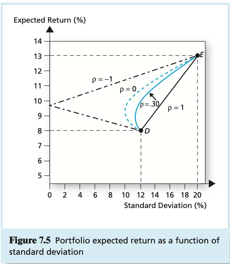
1) Employing Figure 7.5 what are the declining correlation coefficients of 1, 0.3 and then 0 capturing? What direction do you wish to drive the portfolio opportunity sets? Why is that direction important?

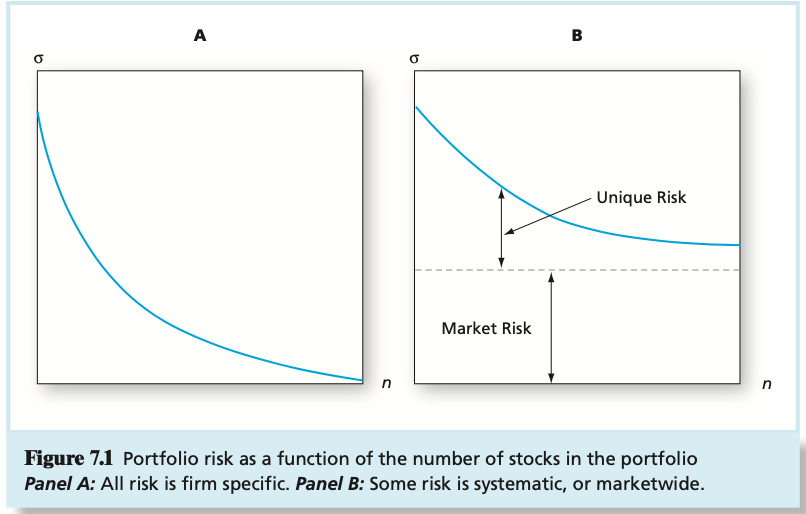
2) Employing Figure 7.1 Panel B what does this panel B convey regarding diversification and its end result? What does it suggest about the risk - and the management of risk - in large n portfolios?

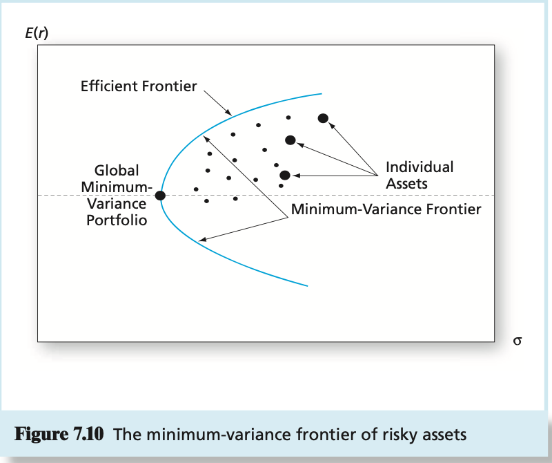
3) Employing Figure 7.10 what do the minimum variance frontier of risky assets and the efficient frontier portray (hint: what makes them different)?

4) Employing Figure 7.8 and Figure 6.8 explain how/why the Risky Portfolio (P) in Figure 6.8 is different from the Risky Portfolio in Figure 7.8?

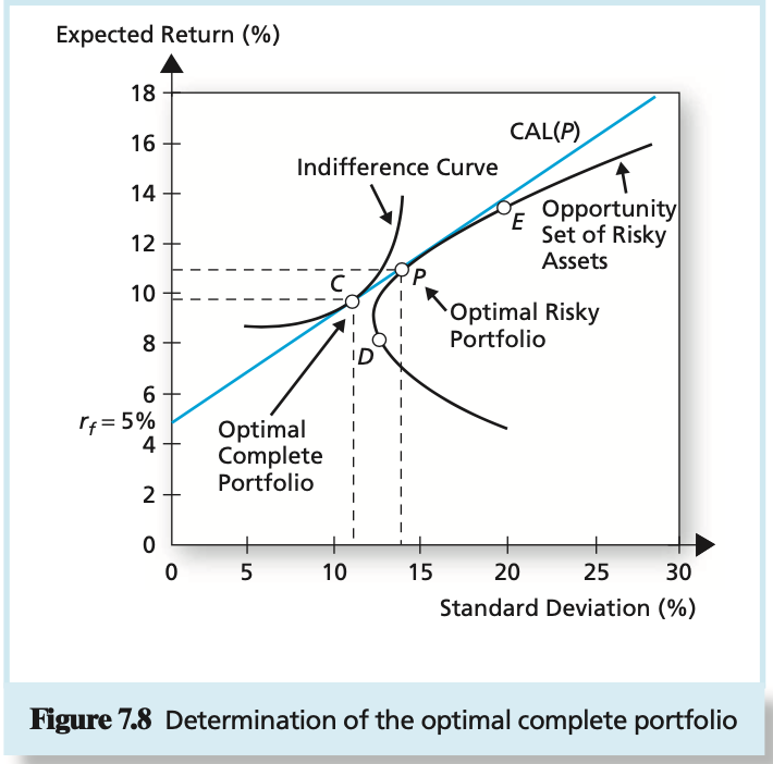
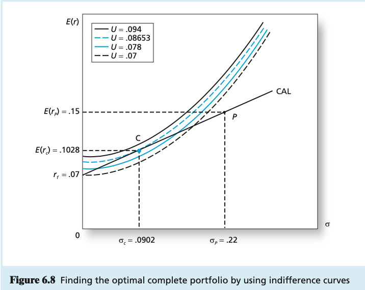
5) Employing Figure 6.8 explain why Portfolio C (client portfolio) is chosen for Client C over Portfolio P (risky portfolio)

Expected Return (%) 14 13 E 12 p=-1 11 p=0 10 p=.30 P=1 9 8 D 74 6 5 0 2 4 6 8 10 12 14 16 18 20 Standard Deviation (%) Figure 7.5 Portfolio expected return as a function of standard deviation B a Unique Risk Market Risk n Figure 7.1 Portfolio risk as a function of the number of stocks in the portfolio Panel A: All risk is firm specific. Panel B: Some risk is systematic, or marketwide. E(r Efficient Frontier Individual Assets Global Minimum- Variance Portfolio Minimum-Variance Frontier 0 Figure 7.10 The minimum-variance frontier of risky assets Expected Return (%) 18 16 14 12 CAL(P) Indifference Curve Opportunity E Set of Risky Assets Optimal Risky Portfolio . 10 8 6 Pf= 5% 4 Optimal Complete Portfolio 2 0 0 5 10 25 15 20 30 Standard Deviation (%) Figure 7.8 Determination of the optimal complete portfolio E(1) U=.094 U= .08653 U=.078 - U=.07 CAL E(r) = .15 Elr) = .1028 ri=.07 o 0 = .0902 On= = .22 Figure 6.8 Finding the optimal complete portfolio by using indifference curves Expected Return (%) 14 13 E 12 p=-1 11 p=0 10 p=.30 P=1 9 8 D 74 6 5 0 2 4 6 8 10 12 14 16 18 20 Standard Deviation (%) Figure 7.5 Portfolio expected return as a function of standard deviation B a Unique Risk Market Risk n Figure 7.1 Portfolio risk as a function of the number of stocks in the portfolio Panel A: All risk is firm specific. Panel B: Some risk is systematic, or marketwide. E(r Efficient Frontier Individual Assets Global Minimum- Variance Portfolio Minimum-Variance Frontier 0 Figure 7.10 The minimum-variance frontier of risky assets Expected Return (%) 18 16 14 12 CAL(P) Indifference Curve Opportunity E Set of Risky Assets Optimal Risky Portfolio . 10 8 6 Pf= 5% 4 Optimal Complete Portfolio 2 0 0 5 10 25 15 20 30 Standard Deviation (%) Figure 7.8 Determination of the optimal complete portfolio E(1) U=.094 U= .08653 U=.078 - U=.07 CAL E(r) = .15 Elr) = .1028 ri=.07 o 0 = .0902 On= = .22 Figure 6.8 Finding the optimal complete portfolio by using indifference curves