1. For HW 11, Problem 1, uncertainties associated with predicting the revenues and cost of manufacturing are estimated to be as follows: (solution for homework 11 problem 1 is given in the photos)

Revenue (price of product): Expected range of variation from base case, low = $45 million, high = $53.5 million.

COMd (raw material cost): Expected range of variation from base case, low = $16 million, high = $21.5 million.

Using the above information, evaluate the expected distribution of NPVs and DCFRORs for the project. Clearly interpret your probability graphs for NPV and DFCROR. Would this analysis change your decision compared to that for the base case?

Note:

a) Use Monte Carlo method in Capcost to complete your analysis. Neatly formatted tables/graphs with additional explanations are mandatory.

b) Because the Monte-Carlo method is based on the generation of random numbers, no two simulations may be exactly the same.

c) Some of the necessary preliminary data (from HW 11, Problem 1) cannot be directly entered into the cells in the Monte-Carlo worksheet in Capcost. They need to be entered step by step in the preceding worksheets (COM Summary, Cash Flow Analysis worksheet, etc.) and the final values will be automatically updated in the Monte-Carlo worksheet.

d) The variations in the percentage range of each factor you wish to analyze may be directly edited in the Monte-Carlo worksheet. Based on the given data for revenue and COMd, manually calculate the % variations on both ends and input the information in Capcost. Set all other factors variations to 0% on both ends.

e) In the Monte Carlo worksheet, you will notice that variations in COMd is not a direct option, depending on which version of CAPCOST is being used. If you are Marcos-savvy, feel free to

rewrite the codes to include COMd variations. If not, input it indirectly using the variations in cost of Raw Material in the COM Summary Worksheet; i.e., set the equation for COMd = Craw materials and input the variability in COMd as a variability in cost of RM. Note that while this is adequate for calculating cumulative cash flow diagrams on the Cash Flow Analysis worksheet, it will not directly work for the Monte Carlo simulation. The reason for this is that the algorithm uses cells C32:C34 to recalculate the COMd during each simulation, regardless of what formula is in cell C36. Therefore, to force the Monte Carlo algorithm to work as desired, cells C32 and C33 should be set to 0, and C34 should be set to 1.

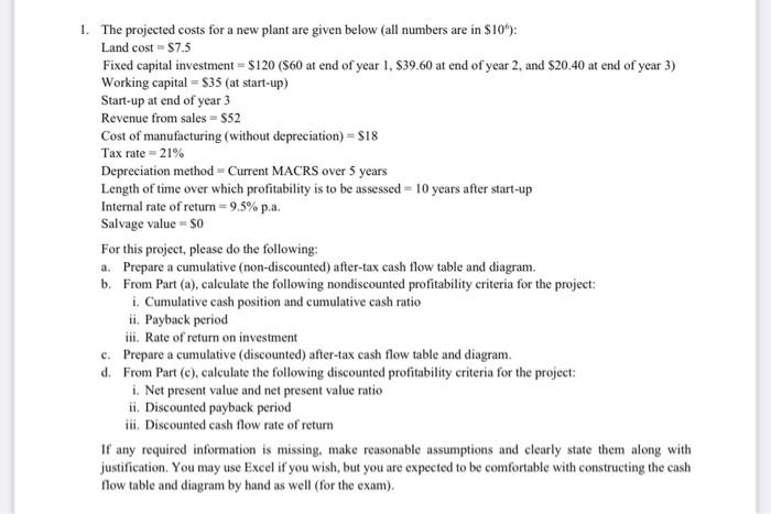
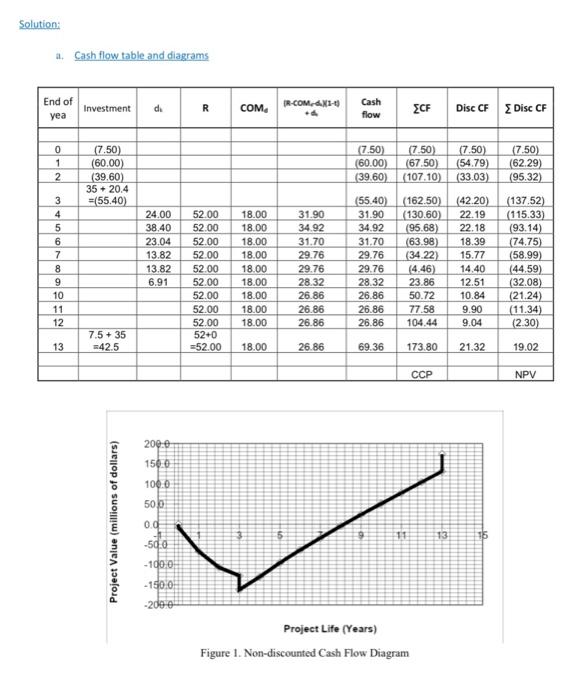
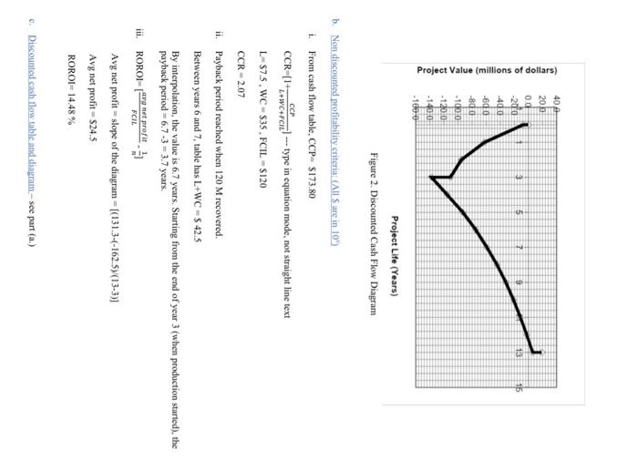
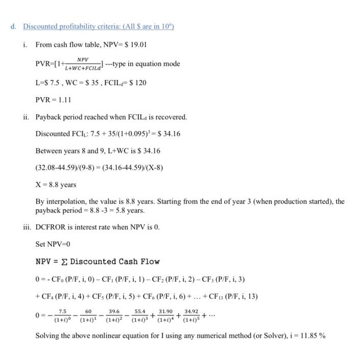
1. The projected costs for a new plant are given below (all numbers are in $106 ): Land cost =$7.5 Fixed capital investment =$120($60 at end of year 1,$39.60 at end of year 2 , and $20.40 at end of year Working capital =$35( at start-up) Start-up at end of year 3 Revenue from sales =$52 Cost of manufacturing (without depreciation) =$18 Tax rate =21% Depreciation method= Current MACRS over 5 years Length of time over which profitability is to be assessed =10 years after start-up Internal rate of return =9.5% p.a. Salvage value =$0 For this project, please do the following: a. Prepare a cumulative (non-discounted) after-tax cash flow table and diagram. b. From Part (a), calculate the following nondiscounted profitability criteria for the project: i. Cumulative cash position and cumulative cash ratio ii. Payback period iii. Rate of return on investment c. Prepare a cumulative (discounted) after-tax cash flow table and diagram. d. From Part (c), calculate the following discounted profitability criteria for the project: i. Net present value and net present value ratio ii. Discounted payback period iii. Discounted cash flow rate of return If any required information is missing. make reasonable assumptions and clearly state them along justification. You may use Excel if you wish, but you are expected to be comfortable with constructing the flow table and diagram by hand as well (for the exam). Solution: a. Cash flow table and diagrams Figure 1. Non-discounted Cash Flow Diagram b. Non discounted profitability criteria: (All $ are in 109 ) i. From cash flow table, CCP=$173.80 CCR=[1+L+WC+PCLCCP] type in equation mode, not straight line text L=$7.5,WC=$35,FClL=$120 CCR=2.07 ii. Payback period reached when 120M recovered. Between years 6 and 7, table has L+WC=$42.5 By interpolation, the value is 6.7 years. Starting from the end of year 3 (when production staried), the payback period =6.73=3.7 years. iii. ROROI =[FCILavgnetprofit=n1] Avg net profit = slope of the diagram =[(131.3(162.5)(133)] Avg net profit =$24.5 ROROI=14.48% c. Discounted cish flow table and diagnm- see part (a.) 1. Discounted profitability criteria: (All \$ are in 106 ) i. From cash flow table, NPV =$19.01 PVR=[1+L+WC+FCILdNPV] type in equation mode L=$7.5,WC=$35,FCILd=$120 PVR =1.11 ii. Payback period reached when FCILd is recovered. Discounted FClL::7.5+35/(1+0.095)3=$34.16 Between years 8 and 9,L+WC is $34.16 (32.0844.59)/(98)=(34.1644.59)/(X8) X=8.8 years By interpolation, the value is 8.8 years. Starting from the end of year 3 (when production started), the payback period =8.83=5.8 years. iii. DCFROR is interest rate when NPV is 0 . Set NPV=0 NPV = Discounted Cash Flow 0=CF0(P/F,i,0)CF1(P/F,i,1)CF2(P/F,i,2)CF3(P/F,i,3) +CF4(P/F,i,4)+CF5(P/F,i,5)+CF6(P/F,i,6)++CF13(P/F,i,13) 0=(1+i)07.5(1+i)160(1+i)239.6(1+i)355.4+(1+i)431.90+(1+i)534.92+ Solving the above nonlinear equation for I using any numerical method (or Solver), i=11.85% 1. The projected costs for a new plant are given below (all numbers are in $106 ): Land cost =$7.5 Fixed capital investment =$120($60 at end of year 1,$39.60 at end of year 2 , and $20.40 at end of year Working capital =$35( at start-up) Start-up at end of year 3 Revenue from sales =$52 Cost of manufacturing (without depreciation) =$18 Tax rate =21% Depreciation method= Current MACRS over 5 years Length of time over which profitability is to be assessed =10 years after start-up Internal rate of return =9.5% p.a. Salvage value =$0 For this project, please do the following: a. Prepare a cumulative (non-discounted) after-tax cash flow table and diagram. b. From Part (a), calculate the following nondiscounted profitability criteria for the project: i. Cumulative cash position and cumulative cash ratio ii. Payback period iii. Rate of return on investment c. Prepare a cumulative (discounted) after-tax cash flow table and diagram. d. From Part (c), calculate the following discounted profitability criteria for the project: i. Net present value and net present value ratio ii. Discounted payback period iii. Discounted cash flow rate of return If any required information is missing. make reasonable assumptions and clearly state them along justification. You may use Excel if you wish, but you are expected to be comfortable with constructing the flow table and diagram by hand as well (for the exam). Solution: a. Cash flow table and diagrams Figure 1. Non-discounted Cash Flow Diagram b. Non discounted profitability criteria: (All $ are in 109 ) i. From cash flow table, CCP=$173.80 CCR=[1+L+WC+PCLCCP] type in equation mode, not straight line text L=$7.5,WC=$35,FClL=$120 CCR=2.07 ii. Payback period reached when 120M recovered. Between years 6 and 7, table has L+WC=$42.5 By interpolation, the value is 6.7 years. Starting from the end of year 3 (when production staried), the payback period =6.73=3.7 years. iii. ROROI =[FCILavgnetprofit=n1] Avg net profit = slope of the diagram =[(131.3(162.5)(133)] Avg net profit =$24.5 ROROI=14.48% c. Discounted cish flow table and diagnm- see part (a.) 1. Discounted profitability criteria: (All \$ are in 106 ) i. From cash flow table, NPV =$19.01 PVR=[1+L+WC+FCILdNPV] type in equation mode L=$7.5,WC=$35,FCILd=$120 PVR =1.11 ii. Payback period reached when FCILd is recovered. Discounted FClL::7.5+35/(1+0.095)3=$34.16 Between years 8 and 9,L+WC is $34.16 (32.0844.59)/(98)=(34.1644.59)/(X8) X=8.8 years By interpolation, the value is 8.8 years. Starting from the end of year 3 (when production started), the payback period =8.83=5.8 years. iii. DCFROR is interest rate when NPV is 0 . Set NPV=0 NPV = Discounted Cash Flow 0=CF0(P/F,i,0)CF1(P/F,i,1)CF2(P/F,i,2)CF3(P/F,i,3) +CF4(P/F,i,4)+CF5(P/F,i,5)+CF6(P/F,i,6)++CF13(P/F,i,13) 0=(1+i)07.5(1+i)160(1+i)239.6(1+i)355.4+(1+i)431.90+(1+i)534.92+ Solving the above nonlinear equation for I using any numerical method (or Solver), i=11.85%