1.)

#include

using namespace std;

void A(char I);

void B(char I);

void match(char t,char I);

int main()

{

char str[50];

cout

cin>>str;

char I;

I=str[0]; // lookahead pointer is assigned to first symbol

A(I);

// if lookahead=$ represents end of the input string

if(I=='$')

cout

return 0;

}

void A(char I)

{

char x,y;

x = 'x';

y = 'y';

if(I=='x')

{

match(x,I);

match(y,I);

B(I);

}

else

{

cout

}

}

void B(char I)

{

char m = 'm';

char n = 'n';

char s = 's';

char t = 't';

if(I=='m')

{

match(m,I);

}

if(I=='n')

{

match(n,I);

}

else if(I=='s')

{

match(s,I);

match(t,I);

}

else

cout

}

void match(char t,char I)

{

if(I=='t')

I=getchar();

else

cout

}

2) code to convert lower case letters to uppercase letters

#include

using namespace std;

int main()

{

char str[50];

cout

cin>>str;

int i;

for(i=0;str[i]!='\0';i++)

{

if(str[i]>='a' && str[i]

{

str[i] = str[i] - 32;

}

}

cout

for(i=0;str[i]!='\0';i++)

{

printf("%c",str[i]);

}

}

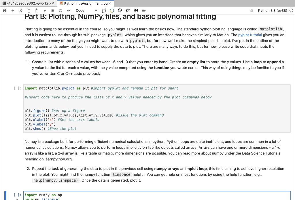
@542ceec59362:-/Workspx PythonIntroAssignment.ipy X a + X O git * - Part B: Plotting, NumPy, files, and basic polynomial fitting Code Python 3.8 (py38) O Plotting is going to be essential in the course, so you might as well learn the basics now. The standard python plotting language is called matplotlib, and it is easiest to use through its sub-package pyplot, which gives you an interface that behaves similarly to Matlab. The pyplot tutorial gives you an introduction to many of the things you might want to do with pyplot, but for now we'll make the simplest possible plot. I've put in the outline of the plotting commands below, but you'll need to supply the data to plot. There are many ways to do this, but for now, please write code that meets the following requirements. 1. Create a list with a series of x values between -6 and 10 that you enter by hand. Create an empty list to store the y values. Use a loop to append a y value to the list for each x value, with the y value computed using the function you wrote earlier. This way of doing things may be familiar to you if you've written C or C++ code previously. [ ]; import matplotlib.pyplot as plt #import pyplot and rename it plt for short #Insert code here to produce the lists of x and y values needed by the plot commands below plt.figure() #set up a figure plt.plot(list_of_x_values, list_of_y_values) #issue the plot command plt.xlabel('x') #Set the axis labels plt.y label('y') plt.show() #Show the plot Numpy is a package built for performing efficient numerical calculations in python. Python loops are quite inefficient, and loops are common in a lot of numerical calculations. Numpy allows you to perform loops implicitly on list-like objects called arrays. Arrays can have one or more dimensions - a 1-d array is like a list, a 2-d array is like a table or matrix; more dimensions are possible. You can read more about numpy under the Data Science Tutorials heading on learnpython.org. 2. Repeat the task of generating the data to plot in the previous cell using numpy arrays an implcit loop, this time aiming to achieve higher resolution in the plot. You might find the numpy function linspace helpful. You can get help on most functions by using the help function, e.g., help(numpy. linspace). Once the data is generated, plot it. [ ]: import numpy as np helninn linsnare help(np. linspace) To focus the telescope we will take measurements of the size of stars at different focus positions and search for the focus position that gives the minimum sized star. The size of the star as a function of focus position is well approximated by a quadratic, so an efficient method of finding the focus is to take a few measurements, fit a quadratic function, and then find its minimum. Here is a table of focus measurements taken previously: Focus position Star size (pixels) -40 4.85 -20 3.71 0 2.56 20 2.51 40 3.17 Create a new CSV (comma separated variable) file by going to the File menu above, clicking "New Launcher," then selecting the "CSV file" app - it will open up a spreadsheet. Add a column and 5 rows, then copy in the values from the table above into the csv file. Save it with a sensible filename (e.g., focus.csv). 3. Write code to load the csv file into a numpy array using the numpy loadtxt function using the optional arguments skiprows=1, delimiter=','. Plot the focus data using stride array indexing to access the individual columns from the csv file (now a 2-d array). You'll want to use a point style formatting for the data points, rather than a line. Don't forget axis labels. [ ]: The points you plotted should look roughly quadratic, so lets fit for the best fit our quadratic function to the data. The curve_fit function in the scipy.optimize package is very easy to use, and has an example of its use at the bottom of its documentation. 4. Fit a quadratic function to the focus data and plot the resulting model as a line in addition to plotting the data on the same plot. Find the minimum of the best fit quadratic curve, either analytically or numerically, and print the focus value and star size at the minimum. []