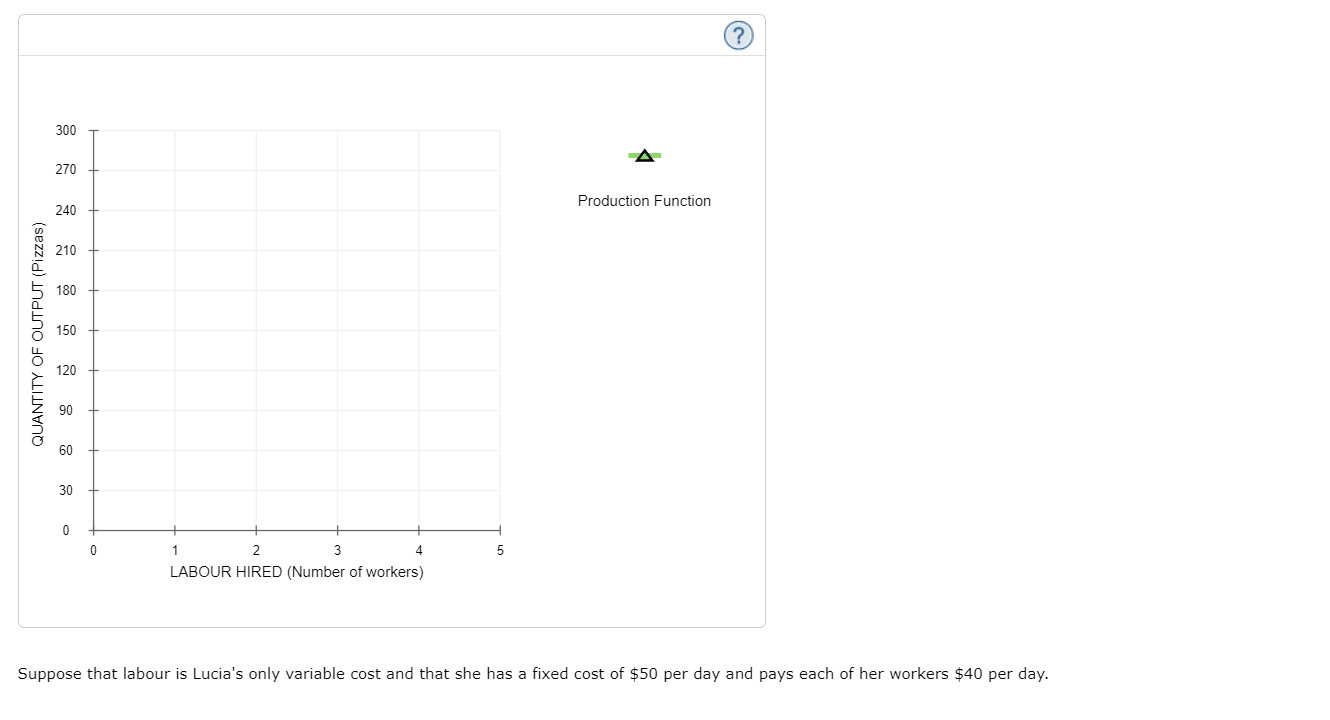
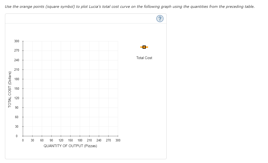
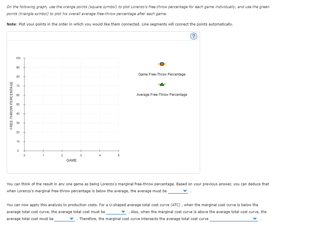
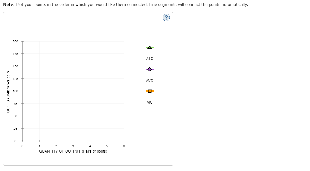
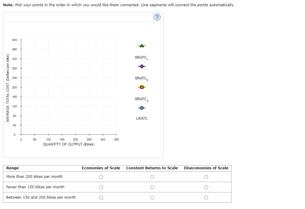
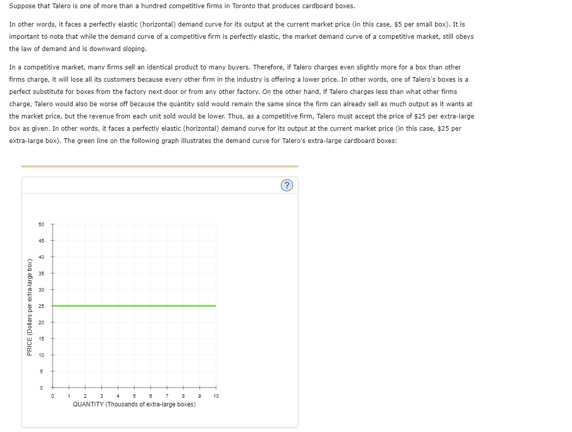
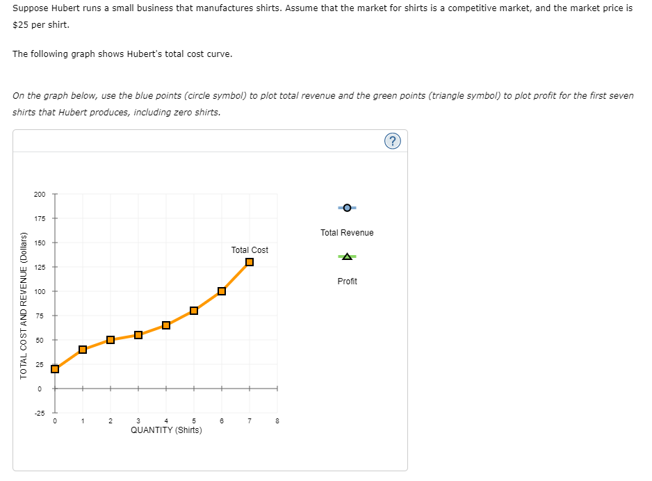
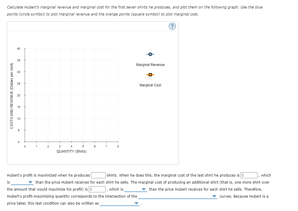
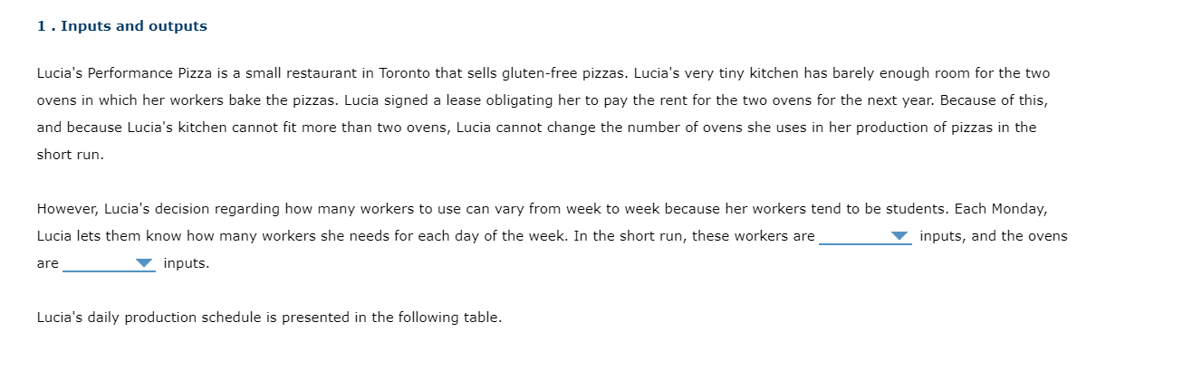
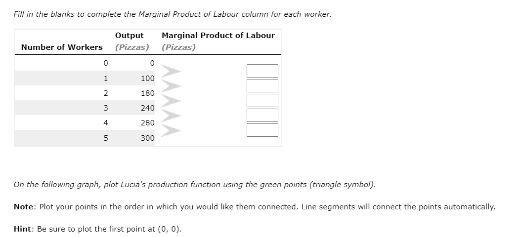
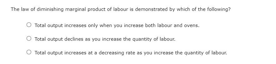
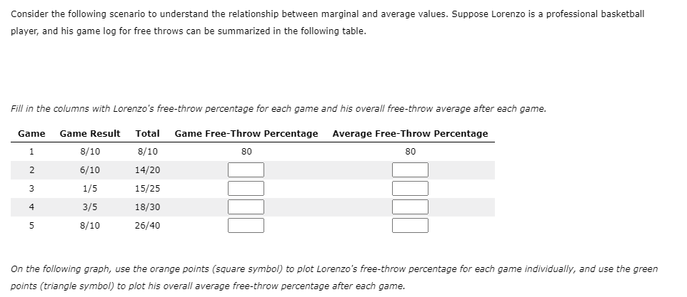
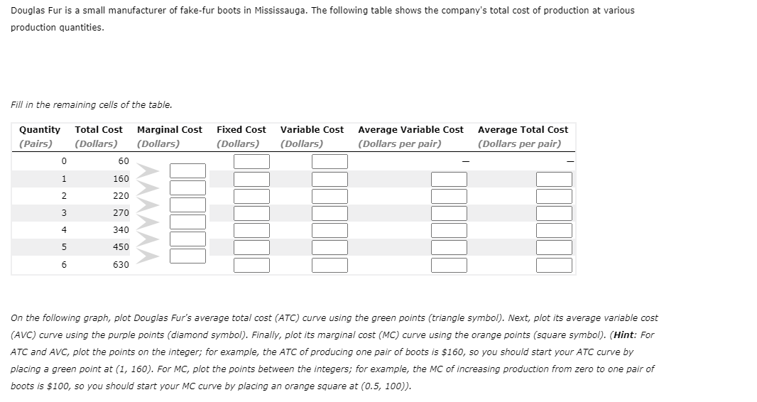
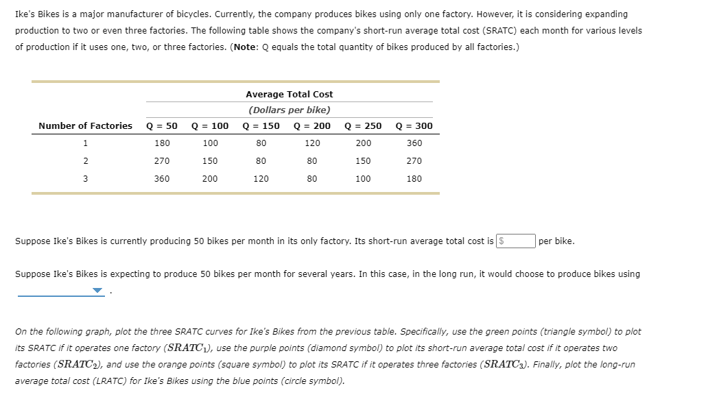
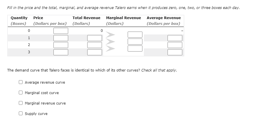
1 . Inputs and outputs Lucia's Performance Pizza is a small restaurant In Toronto that sells gluten-free pizzas. LUCia's very tiny kitchen has barely enough room for the two ovens in which her workers bake the pizzas. Lucia signed a lease obligating her to pay the rent for the two ovens for the next year. Because of thisI and because Lucia's kitchen cannot fit more than two ovens, Lucia cannot change the number of ovens she uses in her production of pizzas in the short run. However, LUCia's decision regarding how many workers to use can vary from week to week because her workers tend to be students. Each Monday, LuCIa lets them know how many workers she needs for each day of the week. In the short run, these workers are 7 inputs, and the ovens are V inputs. Lucia's daily production schedule is presented in the following table. Fill in the blanks to complete the Marginal Product of Labour column for each worker. Output Marginal Product of Labour Number of Workers (Pizzas) (Pizzas) 0 0 100 2 180 3 240 4 280 5 300 On the following graph, plot Lucia's production function using the green points (triangle symbol). Note: Plot your points in the order in which you would like them connected. Line segments will connect the points automatically. Hint: Be sure to plot the first point at (0, 0).300 270 Production Function 240 210 180 QUANTITY OF OUTPUT (Pizzas) 150 120 90 60 30 O 0 1 2 3 LABOUR HIRED (Number of workers) Suppose that labour is Lucia's only variable cost and that she has a fixed cost of $50 per day and pays each of her workers $40 per day.Use the orange points (square symbol) to plot Lucia's total cost curve on the following graph using the quantities from the preceding table. 300 270 Total Cost 240 210 180 150 TOTAL COST (Dollars) 120 90 60 30 30 60 90 120 150 180 210 240 270 300 QUANTITY OF OUTPUT (Pizzas)The law of diminishing marginal product of labour is demonstrated by which of the following? 0 Total output increases only when you increase both labour and ovens. Q Total output declines as you increase the quantity of labour. 0 Total output increases at a decreasing rate as you increase the quantity of labour. Consider the following scenario to understand the relationship between marginal and average values. Suppose Lorenzo is a professional basketball player, and his game log for free throws can be summarized in the following table. Fill in the columns with Lorenzo's free-throw percentage for each game and his overall free-throw average after each game. Game Game Result Total Game Free-Throw Percentage Average Free-Throw Percentage 1 8/10 8/10 80 80 2 6/10 14/20 3 1/5 15/25 4 3/5 18/30 5 8/10 26/40 On the following graph, use the orange points (square symbol) to plot Lorenzo's free-throw percentage for each game individually, and use the green points (triangle symbol) to plot his overall average free-throw percentage after each game.On the following graph, use the orange points (square symbol) to plot torenzo's freethrow percentage for each game individually, and use the green .oofh ts {triangle symbol) to plot his overahI average free throw percentage after each game. Note: Plot your points in the order in which you would like them connected. Line segments will connect the points automatically. 6') 100 -I- go so Game FreeThrow Percentage 70- A on . Average Free-Throw Peroenkige FREE-THROW PERCENTAGE 3 40 30 20 10 g I. . El 1 2 El 4 5 GAME You can think of the result in any one game as being Lorenzo's marginal freethrow percentage. Based on your previous answer, you can deduce that when Lorenzo's marginal freethrow percentage is below the averager the average must be V . You can now apply this analysis to production costs. For a Ushaped average total cost curve {ATCII , when the marginal cost curve is below the average total cost IturveI the average total cost must be V . Also, when the marginal cost curve is above the average total cost curve, the average total cost must be V . Therefore, the marginal cost curve intersects the average total cost curve V . Douglas Fur is a small manufacturer of fakefur boots in Mississauga. The following table shows the company's total cost of production at various production quantities. Fill in the remaining cells of the table. Quantity Total Cost Marginal Cost Fixed Cost Variable Cost Average Variable Cost Average Total Cost { Pairs ,1 (Dollars) {Dollars} (Dollars) (Dollars) (Dollars per pair) (Dollars per pair) 0 60 \\:| E E _ _ 6 630 E E E E On the following graph, plot Douglas Fur's average total cost {ATC} curve using the green ,ooints (triangle symbol). Next, ,olot its average variable cost (AVG) curve using the purple points (diamondI symbol). Finally, plot its marginal cost (MC) curve using the orange points (square symbol). (Hint: For ATC and AFC, plot the points on the integer; for example, the ATC of producing one pair of boots is $1 50, so you should start yourATC curve by placing a green point at (I, 150). For MC, plot the points between the integers; for example, the MC of increasing production from zero to one pair of boots is $100, so you should start your MC curve by placing an orange square at ( o. 5, 1.00)). Note: Plot your points in the order in which you would like them connected. Line segments will connect the points automatically. 200 A 175 ATC 150 125 AVC -0 COSTS (Dollars per pair) 100 MC 75 50 25 1 2 3 QUANTITY OF OUTPUT (Pairs of boots)Ike's Bikes is a major manufacturer of bicycles. Currently, the company produces bikes using only one factory. However, it is considering expanding production to two or even three factories. The following table shows the company's short-run average total cost (SRATC) each month for various levels of production if it uses one, two, or three factories. (Note: Q equals the total quantity of bikes produced by all factories.) Average Total Cost (Dollars per bike) Number of Factories Q = 50 Q = 100 Q = 150 Q = 200 Q = 250 Q = 300 180 100 80 120 200 360 270 150 80 80 150 270 W N 360 200 120 80 100 180 Suppose Ike's Bikes is currently producing 50 bikes per month in its only factory. Its short-run average total cost is $ per bike. Suppose Ike's Bikes is expecting to produce 50 bikes per month for several years. In this case, in the long run, it would choose to produce bikes using On the following graph, plot the three SRATC curves for Ike's Bikes from the previous table. Specifically, use the green points (triangle symbol) to plot its SRATC if it operates one factory (SRATC"), use the purple points (diamond symbol) to plot its short-run average total cost if it operates two factories (SR.ATC2), and use the orange points (square symbol) to plot its SRATC if it operates three factories (SR.ATC:). Finally, plot the long-run average total cost (LRATC) for Ike's Bikes using the blue points (circle symbol).Note: Plot your points in the order in which you would like them connected. Line segments will connect the points automatically. 400 A 380 320 SRATC. 280 240 SRATC2 AVERAGE TOTAL COST (Dollars per bike) 200 160 SRATC, 120 O 80 LRATC 40 50 100 150 200 250 300 350 QUANTITY OF OUTPUT (Bikes) Range Economies of Scale Constant Returns to Scale Diseconomies of Scale More than 200 bikes per month O O O Fewer than 150 bikes per month O O O Between 150 and 200 bikes per month O O OSuppose that Talero is one of more than a hundred competitive rms in Toronto that produces cardboard boxes. In other words, it faces a perfectly elastic [horizontal] demand curve for its output at the current market price (in this case, $5 per small box). It is important to note that while the demand curve of a competitive firm is perfectly elastic, the market demand curve of a competitive market, still obeys the law of demand and is downward sloping. In a competitive market, many rms sell an identical product to many buyers. Therefore, if Talero charges even slightly more for a box than other rms charge, it will lose all its customers because every other lm in the industry is offering a lower price. In other words, one of Talero's boxes is a perfect substitute for boxes from the factory next door or from any other factory. On the other hand, if Talero charges less than what other firms charge, Talero would also be worse off because the quantity sold would remain the same since the rm can already sell as much output as it wants at the market price, but the revenue from each unit sold would be lower. Thus, as a competitive rm, Talero must accept the price of $25 per extralarge box as given. In other words, it faces a perfectly elastic {horizontal} demand curve for its output at the current market price {in this case, $25 per extralarge box]. The green line on the following graph illustrates the demand curve for Talero's extralarge cardboard boxes: (2) 15 PRICE (Dollars per extra-large box) 10 u 1 2 a 4 5 s r s 9 10 QUANTITY (Thousands of extralarge boxes} Fill in the price and the total, marginal, and average revenue Talero earns when it produces zero, one, two, or three boxes each day. Quantity Price Total Revenue Marginal Revenue Average Revenue (Boxes) (Dollars per box) (Dollars) (Dollars) (Dollars per box) 0 0 2 The demand curve that Talero faces is identical to which of its other curves? Check all that apply. Average revenue curve Marginal cost curve Marginal revenue curve O Supply curveSuppose Hubert runs a small business that manufactures shirts. Assume that the market for shirts is a competitive market, and the market price is $25 per shirt. The following graph shows Hubert's total cost curve. On the graph below, use the blue points (circle symbol) to plot total revenue and the green points (triangle symbol) to plot profit for the first seven shirts that Hubert produces, including zero shirts. 200 O 175 Total Revenue 150 Total Cost A 0 125 Profit 100 TOTAL COST AND REVENUE (Dollars) 0 75 0 50 O 1 2 6 7 8 QUANTITY ( Shirts )Calculate Hubert's marginal revenue and marginal cost for the first seven shirts he produces, and plot them on the following graph. Use the blue points (circle symbol) to plot marginal revenue and the orange points (square symbol) to plot marginal cost. 40 O 35 Marginal Revenue 30 25 Marginal Cost COSTS AND REVENUE (Dollars per shirt) 20 15 10 5 3 5 8 7 QUANTITY (Shirts) Hubert's profit is maximized when he produces shirts. When he does this, the marginal cost of the last shirt he produces is $ , which is than the price Hubert receives for each shirt he sells. The marginal cost of producing an additional shirt (that is, one more shirt over the amount that would maximize his profit) is |$ , which is than the price Hubert receives for each shirt he sells. Therefore, Hubert's profit-maximizing quantity corresponds to the intersection of the curves. Because Hubert is a price taker, this last condition can also be written as