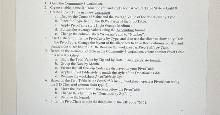
1. Open the Community 3 worksheet. 2. Create a table, name it "Donations2", and apply format White Table Style-Light 8 . 3. Create a PivotTable in a new worksheet a. Display the Count of Value and the average Value of the donations by Type. b. Place the Type field in the ROWS area of the PivotTable. c. Apply PivotTable style Light Orange Medium 4. d. Format the Average values using the Accounting format. e. Change the column labels "Average", and to "Number". 4. Insert a slicer to filter the PivotTable by Type, and then use the slicer to show only Cash in the PivotTable. Change the layout of the slicer box to have three columns. Resize and position the slicer box in E3:H6. Rename the worksheet as PivorTable by Type. 5. Based on the Donations 2 table in the Community 3 worksheet, create another PivotTable in a new worksheet a. Show the Total Value by Zip and by Date in an appropriate format. b. Group the Date by Month. c. Ensure that all five Zip Codes are displayed in your PivotTable. d. Apply a PivotTable style to match the style of the Donations 2 table. e. Rename the worksheet PivotTable by Zip. 6. Based on the PivorTable in the PivotTable by Zip worksheet, create a PivotChart using the 3-D Clustered column chart type. a. Move the PivotChart to the area below the PivotTable. b. Change the chart title to "Donations by Zip". I c. Remove the legend. 7. Filter the PivotChart to hide the donations in the ZIP code 70601