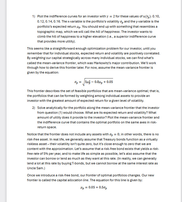
$1)$ Plot the indifference curves for an investor with $\backslash (\backslash$gamma$=2\backslash )$ for these values of $\backslash ($ u$\backslash$left$($r$\_\{$p$\}\backslash$right$)$: $0\mathrm{.}10\backslash ),\backslash (0\mathrm{.}12,0\mathrm{.}14,0\mathrm{.}16\backslash ).$ The x$-$variable is the portfolio's volatility $\backslash (\backslash$sigma$\_\{$p$\}\backslash )$ and the $\backslash ($ y $\backslash )-$variable is the portfolio's expected return $\backslash (\backslash$mu$\_\{$p$\}\backslash ).$ You should end up with something that resembles a topographic map, which we will call the hill of happiness. The investor wants to climb the hill of happiness to a higher elevation $($i$.$e$.,$ a superior indifference curve that provides more utility$).$

This seems like a straightforward enough optimization problem for our investor, until you remember that for individual stocks, expected return and volatility are positively correlated. By weighting our capital strategically across many individual stocks, we can find what's called the mean$-$variance frontier, which was Markowitz's major contribution. We'll work through how to derive this frontier later. For now, assume the mean$-$variance frontier is given by the equation:

$\backslash [$

$\backslash$sigma$\_\{$p$\}=\backslash$sqrt$\{5\backslash$mu$\_\{$p$\}^\{2\}-0\mathrm{.}8\backslash$mu$\_\{$p$\}+0\mathrm{.}05\}$

$\backslash ]$

This frontier describes the set of feasible portfolios that are mean$-$variance optimal; that is$,$ the portfolios that can be formed by weighting among individual assets to provide an investor with the greatest amount of expected return for a given level of volatility.

$2)$ Solve analytically for the portfolio along the mean$-$variance frontier that the investor from question $(1)$ would choose. What are its expected return and volatility? What amount of utility does it provide to the investor? Plot the mean$-$variance frontier and the indifference curve that contains the optimal portfolio on the same axes in riskreturn space.

Notice that the frontier does not include any assets with $\backslash (\backslash$sigma$\_\{$p$\}=0\backslash )$; in other words, there is no risk$-$free asset. In real life, we generally assume that Treasury bonds function as a virtually riskless asset $-$ their volatility isn't quite zero, but it's close enough to zero that we are content with the approximation. Let's assume that a risk$-$free bond exists that yields a riskfree rate of $5\backslash \%$ per year, and to make life as simple as possible, let's also assume that the investor can borrow or lend as much as they want at this rate. $($In reality, we can generally lend a lot at this rate by buying T$-$bonds, but we cannot borrow at the same interest rate as Uncle Sam.$)$

Once we introduce a risk$-$free bond, our frontier of optimal portfolios changes. Our new frontier is called the capital allocation line. The equation for this line is given by:

$\backslash [$

$\backslash$mu$\_\{$p$\}=0\mathrm{.}05+0\mathrm{.}5\backslash$sigma$\_\{$p$\}$

$\backslash ]3)$ Solve analytically for the optimal portfolio chosen by the investor when the capital allocation line is the frontier. What are its expected return and return volatility? How much utility does the investor receive from this portfolio?

$4)$ Plot the mean$-$variance frontier, the capital allocation line, and the indifference curves corresponding to the solutions to $(2)$ and $(3)$ on the same set of axes. Compare the utility from the portfolios in $(2)$ and $(3).$ What is the intuition behind this result? Remember that both solutions are the result of solving a constrained optimization problem.

There is one portfolio that sits on both the mean$-$variance frontier and the capital allocation line. We call this portfolio the tangency portfolio, and it's important because it turns out that we can create any portfolio along the capital allocation line by combining just two assets: a risk$-$free debt position $($either borrowing or lending$)$ and a position in a mutual fund that mimics the tangency portfolio. This is known as the two$-$fund theorem in asset pricing. Portfolios along the capital allocation line to the left of the tangency portfolio are said to be in the lending region of the frontier, and consist of long positions $($i$.$e$.,$ positive weights$)$ on both the risk$-$free debt asset and the risky mutual fund. Portfolios along the capital allocation line to the right of the tangency portfolio are said to be in the borrowing region and consist of a short position in the risk$-$free debt asset and a long position in the risky mutual fund. The weight on the debt position will be negative and the weight on the risky mutual fund will be greater than one; conceptually, you are investing more than $\backslash (100\backslash \%\backslash )$ of your available capital by borrowing additional funds at the risk$-$free rate.

$5)$ Find the expected return and return variance of the tangency portfolio. Then, find the weights of the risk$-$free bond and the risky mutual fund that replicates the tangency portfolio in the optimal portfolio that solves $(3).$

$6)$ There is an investor with a utility function $\backslash ($ u$\backslash$left$($r$\_\{$p$\}\backslash$right$)=\backslash$mu$\_\{$p$\}-\backslash$gamma$\_\{$t$\}\backslash$sigma$\_\{$p$\}^\{2\}\backslash )$ for whom the tangency portfolio is optimal. What is this investor's risk aversion coefficient $\backslash (\backslash$gamma$\_\{$t$\}\backslash )?$ Revisit your answer to question $(4).$ What can you say about this investor in the context of constrained optimization and the way in which we've altered the constraint on the problem between question $(2)$ and $(3)?$