$1$ Start Excel. Open the downloaded file named Excel$\_$CH$13\_$PS$1\_$Metrics.xlsx$.$ Grader has automatically added your last name to the beginning of the filename. Save the file to the location where you are storing your files.

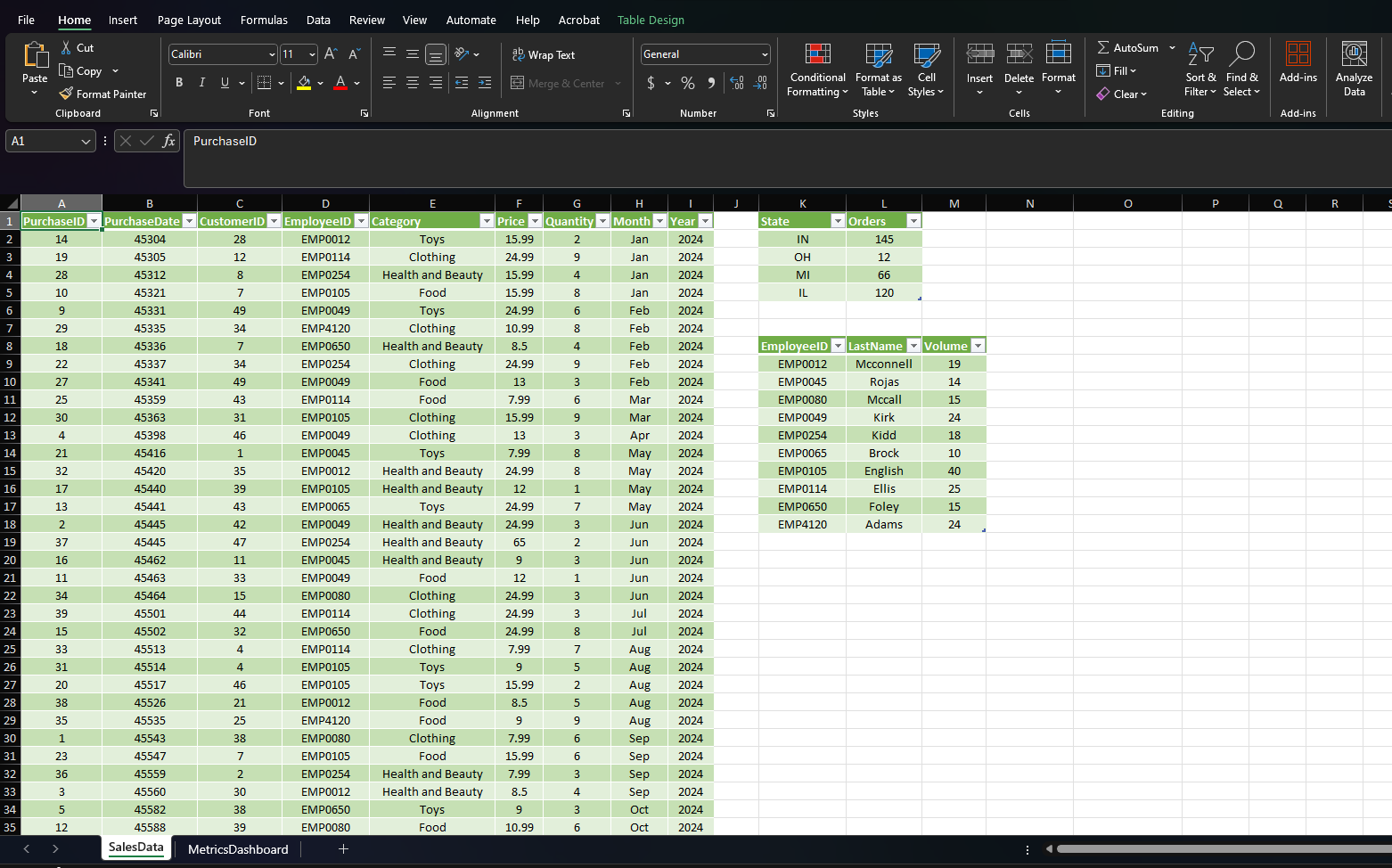
$2$ On the SalesData worksheet, use the Geography Data Type to view the corresponding Population for each of the states listed in the table.

$3$ To build an interactive dashboard from multiple tables, each table must first be added to the data model.

On the SalesData worksheet tab, add each of the tables to the data model.

$4$ Edit the data model by completing the following tasks on the SalesData worksheet:

Format the PurchaseDate field as $*3/14/2012$

Format the Price field as Currency

$5$ On the SalesData$2024$ Power Pivot tab, create a calculated column to the right of Year with the name Revenue. Use the formula $=[$Price$]*[$Quantity$]$ to calculate the revenue generated from each sale. Format the column as Currency, $ English $($United States$).$

$6$ In Power Pivot, create a calculated field for sum of revenue in the Calculation Area just below the Revenue column. Ensure that the name of the measure $($the text before the colon$)$ is Sum of Revenue. Copy the calculated field and paste it as text into cell A$1$ of the MetricsDashboard worksheet in the main workbook.

From the Power Pivot window, create a KPI that measures the Sum of Revenue value against the absolute value of $$500\mathrm{.}00.$ Maintain the default thresholds of $200$ and $400$ and select the fourth set of icon styles.

Create a relationship between SalesData$2024$ and VolumeByEmp using the EmployeeID field.

$7$ In the Power Pivot window, create a Chart and Table $($Horizontal$)$ combination on the MetricsDashboard worksheet in cell B$2.$ In the PivotChart, drag the Category field from SalesData$2024$ to the Axis $($Categories$)$ area. Drag the Quantity field from SalesData$2024$ to the Values area to calculate the sum of quantity sold.

Change the chart type to a Pie chart. Apply Style $9$ to the PivotChart. Add a Chart Title that reads Volume Sales by Category.

Add a Timeline slicer connected to the PivotChart, select the PurchaseDate check box, and position it below the chart. Apply the Light Green, Timeline Style Light $6$ to the slicer.

$8$ Name the PivotTable EmployeeRevGoals. Drag the LastName field from VolumeByEmp to the Rows area. Drag the Sum of Revenue Value field from SalesData$2024$ to the Values area. Drag the Sum of Revenue KPI Status field to the Values area.

Rename the Row Labels heading in J$2$ to Employees. Rename the Sum of Revenue heading in K$2$ to $2024$ Revenue. Rename the Sum of Revenue Status heading in L$2$ as $$500$ Goal Status. If necessary, resize the column to fit the text. Apply the PivotTable Style, Light Green, Pivot Style Medium $14$ to the PivotTable.

$9$ From the Power Pivot window, create a PivotTable on the MetricsDashboard worksheet in cell B$25.$ Drag the State field from OrdersByState to the Rows area and the Orders field to the Values area. Convert the PivotTable to formulas. Change the label in cell B$25$ to State.

$10$ Insert a Filled Map chart to the MetricsDashboard worksheet using cells B$25$:C$29,$ and complete the following. Change the chart title to Number of Orders by State. Position the map within the cell range B$25$:H$39.$

$11$ From the OrdersbyState Power Pivot window, create a second PivotTable on the MetricsDashboard worksheet in cell I$25.$ Drag the State field from OrdersByState to the Rows area and the Population field to the Values area. Convert the PivotTable to formulas.

$12$ Insert a second Filled Map chart to the MetricsDashboard worksheet using cells I$25$:J$29,$ and complete the following. Change the chart title to Population by State. Position the map within the cell range I$25$:M$39.$

$13$ Prepare the dashboard for production by hiding the SalesData worksheet. Hide the column and row headings as well as the gridlines on the MetricsDashboard worksheet.

$14$ Minimize the ribbon. Protect the worksheet, allowing only to Use PivotTable & PivotChart and Edit objects.