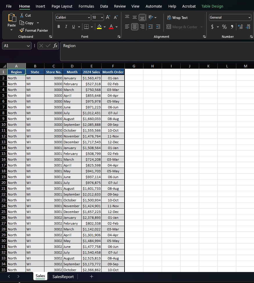
$1$ Start Excel. Open the downloaded file named Excel$\_$CH$13\_$PS$2\_$PaperSales.xlsx$.$ Grader has automatically added your last name to the beginning of the filename. Save the file to the location where you are storing your files. $0$

$2$ On the Sales worksheet, with cell A$1$ selected, display the Power Pivot tab, and then in the Tables group, click or press Add to Data Model. $14$

$3$ Close the Power Pivot for Excel window. Display the SalesReport worksheet. Type Paper Mill Sales Report in cell A$1,$ changing the font to $18$ pt and bold. $4$

$4$ Insert a PivotChart into the worksheet using the workbook's Data Model as the source. Move the PivotChart so that the upper$-$left corner of the chart is in cell B$2$ and the lower$-$right corner of the PivotChart is in I$16.8$

$5$ Add $2024$ Sales as the Value and Month Order as the Axis. Ensure the chart is a Clustered Column chart. If necessary, remove the legend. Add the chart title $2024$ Sales by Month to the PivotChart. $12$

$6$ Insert a second PivotChart into the worksheet using the workbook's Data Model as the source. Move the PivotChart so that the upper$-$left corner of the chart is in cell J$2$ and the lower$-$right corner of the PivotChart is in Q$16.8$

$7$ Add $2024$ Sales as the Value and Month Order as the Axis. Add Region as the Legend. Change the chart type to a Line with Markers chart. Add the chart title $2024$ Sales by Region to the PivotChart. $18$

$8$ Insert a PivotTable into cell C$21$ on the worksheet using the workbook's Data Model as the source. Add State as the Row and $2024$ Sales for the Values. Remove the Grand Totals for both Rows and Columns. $8$

$9$ Insert a slicer for Month Order. Move the Slicer so that the upper$-$left corner is in cell J$21$ and the lower$-$right corner of the Slicer is in L$40.8$

$10$ Convert the PivotTable to Formulas. Insert a Filled Map Chart using the converted PivotTable. Type $2024$ Sales by State as the chart title. Move the Chart so that the upper$-$left corner of the chart is in cell C$21$ and the lower$-$right corner of the chart is in I$35.12$

$11$ Hide the Gridlines and Headings on the worksheet. $8$

$12$ Save and close Excel$\_$CH$13\_$PS$2\_$PaperSales. Exit Excel. Submit the file as directed. $0$