Question: 1. Use the dataset HP.txt to set up a multiple linear regression and do some assumptions analy- sis. The dataset contains information on 100 homes

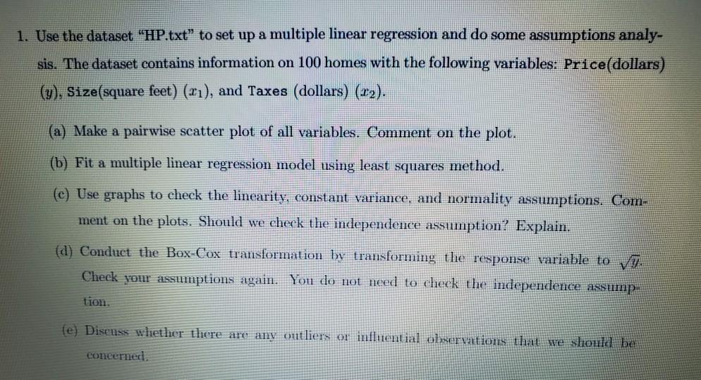
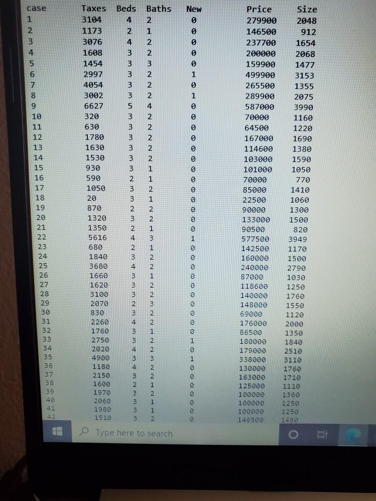
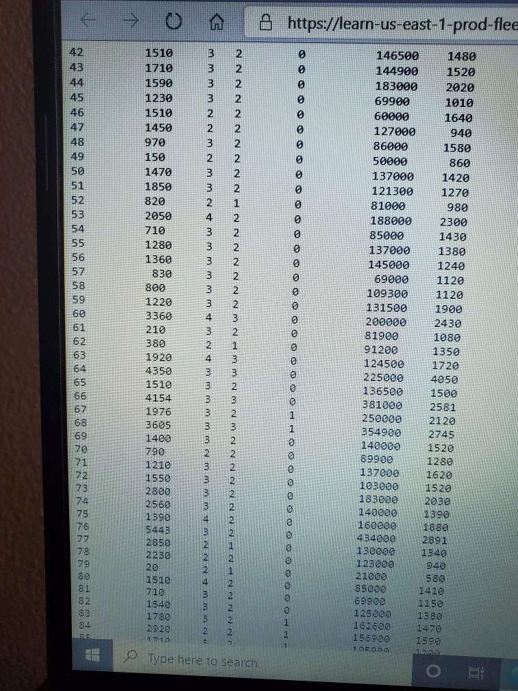
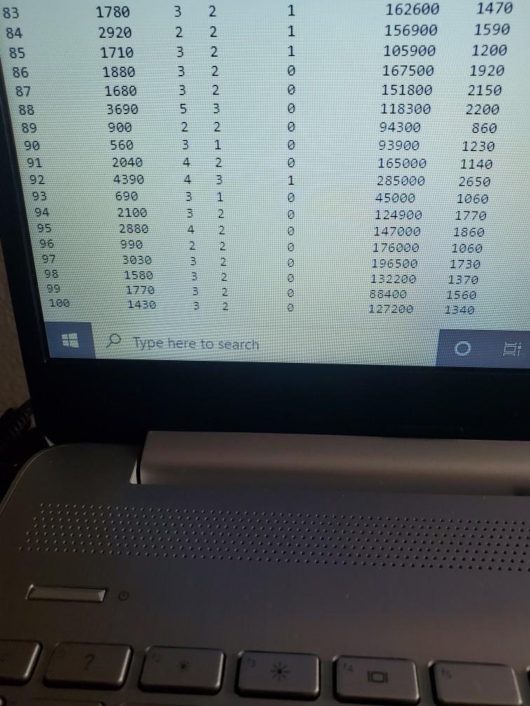
1. Use the dataset "HP.txt" to set up a multiple

1. Use the dataset "HP.txt" to set up a multiple linear regression and do some assumptions analy- sis. The dataset contains information on 100 homes with the following variables: Price(dollars) (y), Size(square feet) (x1), and Taxes (dollars) (x2). (a) Make a pairwise scatter plot of all variables. Comment on the plot. (b) Fit a multiple linear regression model using least squares method. (e) Use graphs to check the linearity, constant variance, and normality assumptions. Com- ment on the plots. Should we check the independence assumption? Explain. (d) Conduct the Box-Cox transformation by transforming the response variable to . Check your assumptions again. You do not need to check the independence assurnp tion (e) Discuss whether there are any outliers or influential observations that we should be concerned. case 1 New 0 0 9 0 0 1 9 1 0 0 0 0 0 0 0 0 0 2 3 4 5 6 7 8 9 10 11 12 13 14 15 16 17 18 19 20 21 22 23 24 25 26 27 28 29 30 31 32 33 34 35 36 37 38 39 40 41 42 Taxes 3104 1173 3076 1608 1454 2997 4054 3002 6627 320 630 1780 1630 1530 930 590 1050 20 870 1320 1350 5616 680 1840 3680 1660 1620 3100 2070 830 2260 1760 2750 2020 4900 1180 2150 1600 1970 2060 1980 1510 Beds Baths 4 2 2 1 4 2 3 2 3 3 3 2 3 2 3 2 5 4 3 2 3 2 3 2 3 2 3 2 3 1 2 1 3 2 3 1 2 2 3 2 2 1 4 3 2 1 3 2 4 2 3 1 3 2 3 2 2 3 3 2 4 2 3 1 3 2 4 2 3 3 4 2 3 2 2 1 3 2 3 1 3 1 3 Price Size 279900 2048 146500 912 237700 1654 200000 2068 159900 1477 499900 3153 265500 1355 289900 2075 587099 3990 70000 1160 64500 1220 167000 1690 114600 1380 103000 1590 101000 1050 70000 770 85000 1410 22500 1060 90000 1300 133000 1500 90500 820 577500 3949 142500 1170 160000 1500 240000 2790 87000 1030 118600 1250 140000 1760 148000 1550 69000 1129 176000 2000 86500 1350 180000 1840 179000 2510 338000 3110 130000 1760 163000 1710 125000 1110 100000 1360 100000 1250 100080 1250 146500 1480 0 1 @ 0 0 3 1 @ 1 @ @ Type here to search > 0 @ https://learn-us-east-1-prod-flee 2 2 2 2 2 2 2 42 43 44 45 46 47 48 49 50 51 52 53 54 55 56 57 58 59 60 61 62 63 64 65 66 67 68 69 70 71 72 73 74 75 76 77 3 3 3 3 2 2 3 2 3 3 2 4 3 3 3 3 3 3 4 3 2 4 3 3 3 3 3 3 2 3 5 3 3 2 2 1510 1710 1590 1230 1510 1450 970 150 1470 1850 820 2050 710 1280 1360 830 800 1220 3360 210 380 1920 4350 1510 4154 1976 3605 1400 790 1210 1550 2800 2560 1390 5443 2850 2230 20 1510 710 1540 1780 2920 1718 1480 1520 2020 1010 1640 940 1580 860 1420 1270 980 2300 1430 1380 1240 1120 1120 1900 2430 1080 1350 2 3 2 1 @ 146500 144900 183000 69900 60000 127000 86000 50000 137000 121300 81000 188000 85000 137000 145000 69000 109300 131500 200000 81900 91200 124500 225000 136500 381000 250000 354900 140000 89900 137000 103000 185000 140000 160000 434000 130000 123000 21000 85000 69900 125000 162609 156900 1 aaaa e 1720 @ 0 1 4050 1500 2581 2120 2745 1520 1280 1620 1520 2030 1390 1880 2891 1340 940 580 1410 1150 1380 1470 1590 15 3 79 80 4 3 82 83 84 2 Type here to search 1 1 1 83 84 85 86 87 88 89 1780 2920 1710 1880 1680 3690 NNNNNm Nanma NN NN No mnm mm innm+ + m mmmmm 560 2040 4390 690 2100 2880 990 3030 1580 1770 1430 91 92 93 94 95 96 97 98 99 100 4 1 162600 1470 156900 1590 105900 1200 167500 1920 151800 2150 118300 2200 94300 860 93900 1230 165000 1140 285000 2650 45000 1060 124900 1770 147000 1860 176000 1060 196500 1730 132280 1370 88400 1560 127202 ooooo 0 0 @ @ @ @ @ @ Type here to search 1. Use the dataset "HP.txt" to set up a multiple linear regression and do some assumptions analy- sis. The dataset contains information on 100 homes with the following variables: Price(dollars) (y), Size(square feet) (x1), and Taxes (dollars) (x2). (a) Make a pairwise scatter plot of all variables. Comment on the plot. (b) Fit a multiple linear regression model using least squares method. (e) Use graphs to check the linearity, constant variance, and normality assumptions. Com- ment on the plots. Should we check the independence assumption? Explain. (d) Conduct the Box-Cox transformation by transforming the response variable to . Check your assumptions again. You do not need to check the independence assurnp tion (e) Discuss whether there are any outliers or influential observations that we should be concerned. case 1 New 0 0 9 0 0 1 9 1 0 0 0 0 0 0 0 0 0 2 3 4 5 6 7 8 9 10 11 12 13 14 15 16 17 18 19 20 21 22 23 24 25 26 27 28 29 30 31 32 33 34 35 36 37 38 39 40 41 42 Taxes 3104 1173 3076 1608 1454 2997 4054 3002 6627 320 630 1780 1630 1530 930 590 1050 20 870 1320 1350 5616 680 1840 3680 1660 1620 3100 2070 830 2260 1760 2750 2020 4900 1180 2150 1600 1970 2060 1980 1510 Beds Baths 4 2 2 1 4 2 3 2 3 3 3 2 3 2 3 2 5 4 3 2 3 2 3 2 3 2 3 2 3 1 2 1 3 2 3 1 2 2 3 2 2 1 4 3 2 1 3 2 4 2 3 1 3 2 3 2 2 3 3 2 4 2 3 1 3 2 4 2 3 3 4 2 3 2 2 1 3 2 3 1 3 1 3 Price Size 279900 2048 146500 912 237700 1654 200000 2068 159900 1477 499900 3153 265500 1355 289900 2075 587099 3990 70000 1160 64500 1220 167000 1690 114600 1380 103000 1590 101000 1050 70000 770 85000 1410 22500 1060 90000 1300 133000 1500 90500 820 577500 3949 142500 1170 160000 1500 240000 2790 87000 1030 118600 1250 140000 1760 148000 1550 69000 1129 176000 2000 86500 1350 180000 1840 179000 2510 338000 3110 130000 1760 163000 1710 125000 1110 100000 1360 100000 1250 100080 1250 146500 1480 0 1 @ 0 0 3 1 @ 1 @ @ Type here to search > 0 @ https://learn-us-east-1-prod-flee 2 2 2 2 2 2 2 42 43 44 45 46 47 48 49 50 51 52 53 54 55 56 57 58 59 60 61 62 63 64 65 66 67 68 69 70 71 72 73 74 75 76 77 3 3 3 3 2 2 3 2 3 3 2 4 3 3 3 3 3 3 4 3 2 4 3 3 3 3 3 3 2 3 5 3 3 2 2 1510 1710 1590 1230 1510 1450 970 150 1470 1850 820 2050 710 1280 1360 830 800 1220 3360 210 380 1920 4350 1510 4154 1976 3605 1400 790 1210 1550 2800 2560 1390 5443 2850 2230 20 1510 710 1540 1780 2920 1718 1480 1520 2020 1010 1640 940 1580 860 1420 1270 980 2300 1430 1380 1240 1120 1120 1900 2430 1080 1350 2 3 2 1 @ 146500 144900 183000 69900 60000 127000 86000 50000 137000 121300 81000 188000 85000 137000 145000 69000 109300 131500 200000 81900 91200 124500 225000 136500 381000 250000 354900 140000 89900 137000 103000 185000 140000 160000 434000 130000 123000 21000 85000 69900 125000 162609 156900 1 aaaa e 1720 @ 0 1 4050 1500 2581 2120 2745 1520 1280 1620 1520 2030 1390 1880 2891 1340 940 580 1410 1150 1380 1470 1590 15 3 79 80 4 3 82 83 84 2 Type here to search 1 1 1 83 84 85 86 87 88 89 1780 2920 1710 1880 1680 3690 NNNNNm Nanma NN NN No mnm mm innm+ + m mmmmm 560 2040 4390 690 2100 2880 990 3030 1580 1770 1430 91 92 93 94 95 96 97 98 99 100 4 1 162600 1470 156900 1590 105900 1200 167500 1920 151800 2150 118300 2200 94300 860 93900 1230 165000 1140 285000 2650 45000 1060 124900 1770 147000 1860 176000 1060 196500 1730 132280 1370 88400 1560 127202 ooooo 0 0 @ @ @ @ @ @ Type here to search

Step by Step Solution

There are 3 Steps involved in it

1 Expert Approved Answer

Step: 1 Unlock blur-text-image

Question Has Been Solved by an Expert!

Get step-by-step solutions from verified subject matter experts

Step: 2 Unlock

Step: 3 Unlock

Students Have Also Explored These Related General Management Questions!

for this problem I just want to know for part(a)how to make a pair wise scatter plot of all variables on R. also describe for me how to do part(c) using R as well. thanks. . Use the dataset "HP.txt"...

Data Exploration and Multiple Linear Regression (MLR) using SAS. The College data set contains the statistics for many US Colleges from 1995 issue of US News and World Report. It has 777 observations...

Q9some type is wrong, can refer to the attach file. In a study of the relationship between an explanatory variable Z and a response variable Y , n independent observations are taken in the form of...

Specification and Verification II Consider the following Verilog phrases: initial r = 0; always @(posedge clk) r = a + r; Write down a formula in logic that relates clk, a and r at a level of...

Discussion Board Week 2 1. "Estimating Demand and Its Elasticities" and Statistical Estimation of the Demand Curve During the Weekly Scenarios Herb Jones, a graduate student and part-time data...

1) What are your five key takeaways (what did you find interesting, what surprised you, etc)? Provide details for each takeaway. - Using Tables 1-4 (on pages 7 and 8), what information could you...

ACCT 326 Writing Assignment #1 Managing in a global, digital society requires accountants to pay close attention about information. One of the reasons accountants have to pay close attention to...

6.1 Predicting Boston Housing Prices. The file Boston Housing.csy contains informa- tion collected by the US Bureau of the Census concerning housing in the area of Boston, Massachusetts. The dataset...

IN DESPERATE NEED OF HELP FOR THIS PROJECT. TRIED TO GET IT TO WORK AND MY REGRESSION IN EXCEL WOULDNT. PLEASE HELP of 7 ZOOM + Statistical Research Projects Project Objective: Application...

Link to data required attached below https://drive.google.com/drive/folders/1LTx-MVOBQgFrLwrl1fe5EtZK4GfaenB7?usp=sharing Homework 10: Multiple Linear Regression NAME: Your Name NETID: Your NetID DUE...

The comparative balance sheets for Novak Corporation show the following information. December 31 2020 2019 Cash $33,700 $13,200 Accounts receivable 12,100 9,900 Inventory 12,000 9,100...

Kipper Company made the following data available from its accounting records and reports: (a) $800,000 estimated factory overhead/200,000 estimated machine hours = $4 predetermined factory overhead...

Non - accelerated filers must file in how many days from fiscal year - end?

When older adults have difficulty with transportation and communication, or may be reluctant to request needed assistance to which they are entitled, they may be in need of: Group of answer choices...