1) When testing a null hypothesis against the alternative, the p-value tells us ______

Whether the test is a one tailed or two-tailed test

Whether the null is appropriately constructed

To reject the null if the p-value is less than the significance level

Whether the significance level should be changed

2) "Students receiving a 4.0 in their first semester of college don't work as hard in future semesters, explaining why the GPAs of that group of students fall over their college career." This statement is an example of ____

Homer Simpson's paradox.

the regression fallacy.

regression to mediocrity.

the gambler's fallacy.

3

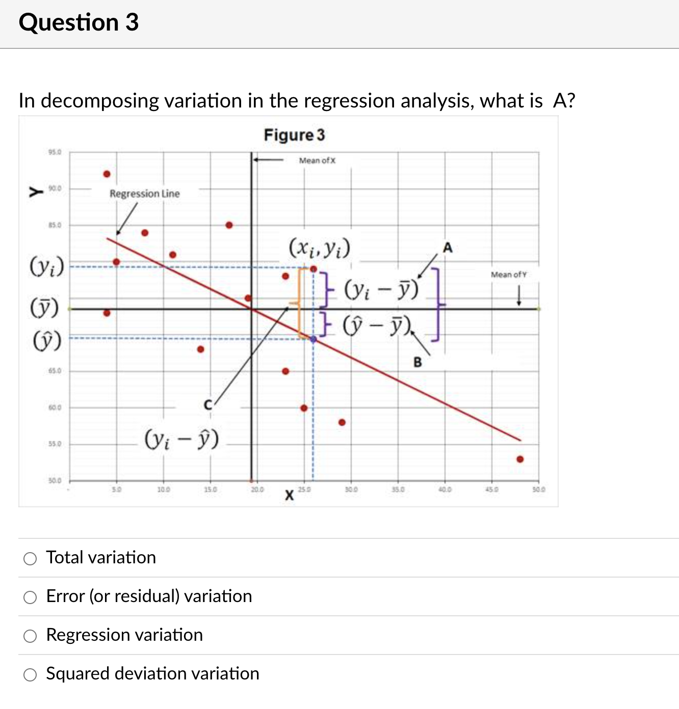
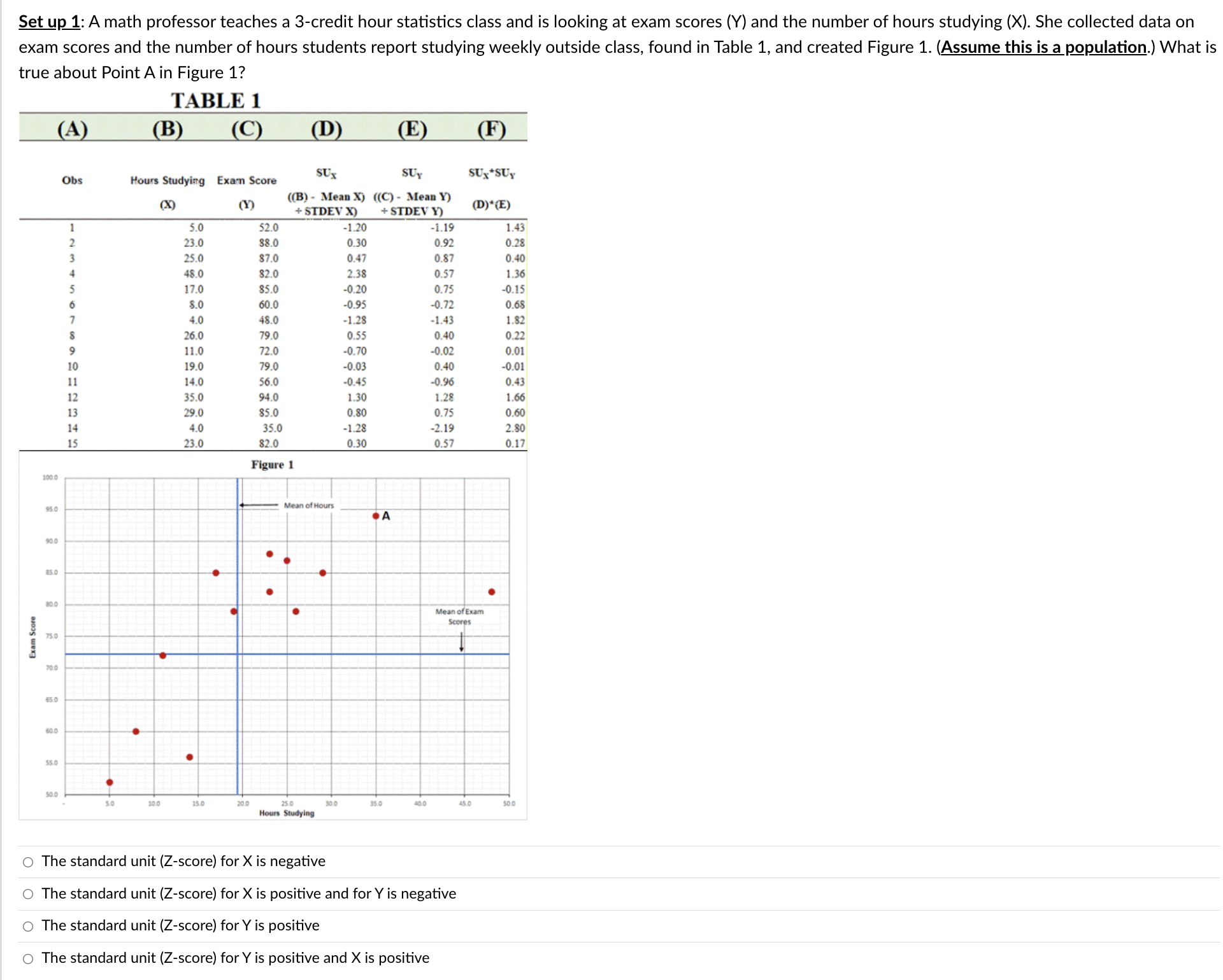
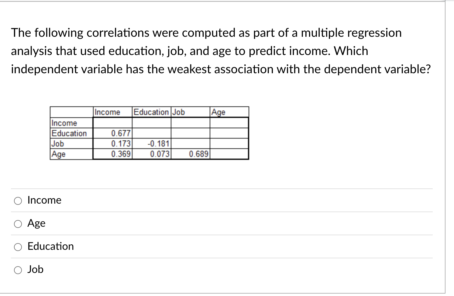
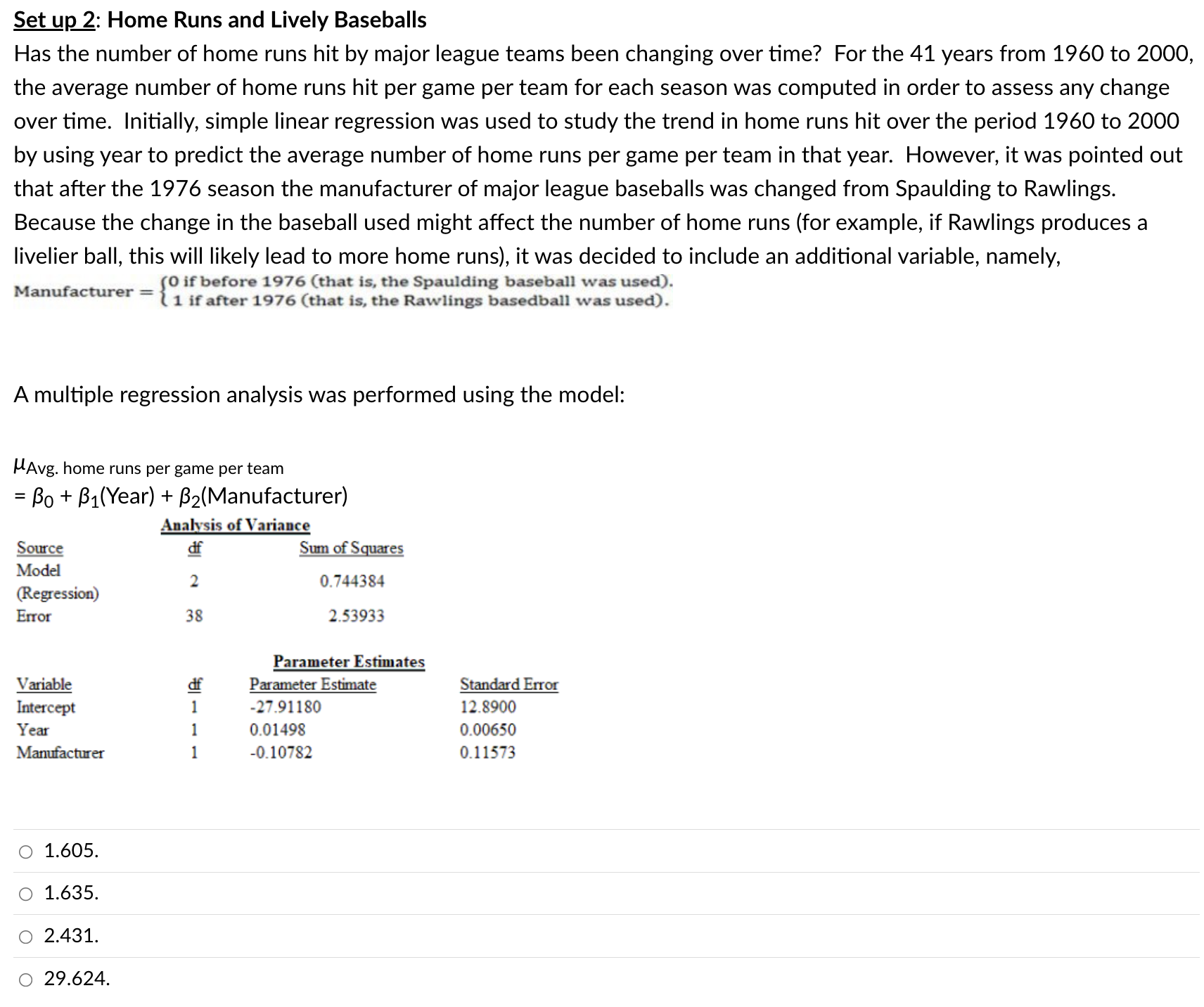
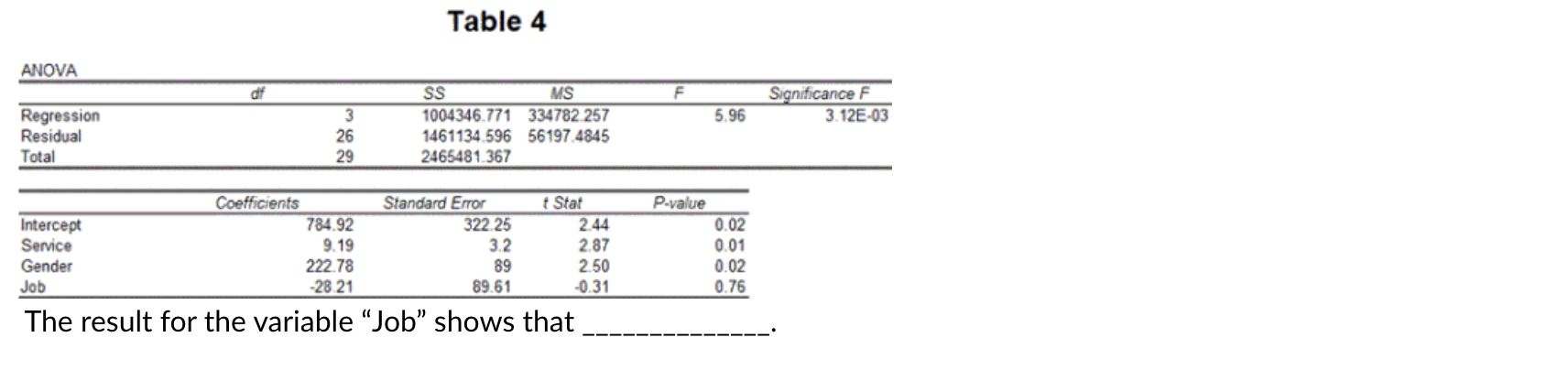
Question 3 In decomposing variation in the regression analysis, what is A? 0 Total variation 0 Error (or residual) variation 0 Regression variation 0 Squared deviation variation The following correlations were computed as part of a multiple regression analysis that used education, job, and age to predict income. Which independent variable has the weakest association with the dependent variable? Income Education Job Age Income Education 0.677 Job 0.173 -0. 181 Age 0.369 0.073 0.689 O Income O Age O Education O JobSet up 1: A math professor teaches a 3-credit hour statistics class and is looking at exam scores (Y) and the number of hours studying (X). She collected data on exam scores and the number of hours students report studying weekly outside class, found in Table 1, and created Figure 1. (Assume this is a population.) What is true about Point A in Figure 1? TABLE 1 (A) (B (C (D (E) (F) SUX SUy SUx *SUY Obs Hours Studying Exam Score ((B) - Mean X) ((C) - Mean Y) (X) (Y) + STDEV Y) (D)*(E) + STDEV X) 3.0 52.0 -1.20 -1.19 1.43 23.0 $8.0 0.30 0.92 0.28 AWN - 25.0 $7.0 0.47 0.87 0.40 48.0 82.0 2.38 0.57 1.36 17.0 35.0 -0.20 0.75 0.15 $.0 60.0 -0.95 -0.72 0.68 4.0 48.0 -1.28 -1.43 1.82 26.0 79.0 0.55 0.40 0.22 11.0 72.0 -0.70 0.02 0.01 19.0 79.0 -0.03 0.40 -0.01 14.0 56.0 0.45 -0.96 0.43 35.0 94.0 1.30 1.28 1.66 29.0 35.0 0.80 0.75 0.60 4.0 35.0 -1.28 -2.19 2.80 23.0 32.0 0.30 0.57 0.17 Figure 1 100 0 95 0 A 90 0 85.0 80.0 Mean of Exam Scores Exam Score 75.0 20.0 65 0 60.0 SS.0 30.0 15.0 20.0 30 0 35 0 45.0 Hours Studying O The standard unit (Z-score) for X is negative O The standard unit (Z-score) for X is positive and for Y is negative O The standard unit (Z-score) for Y is positive O The standard unit (Z-score) for Y is positive and X is positiveA sales manager for an advertising agency believes that there is a relationship between the number of contacts (with prospective clients) and the amount of sales dollars earned. A regression analysis shows the following results ____ Standard Error m Maine 0. 100 Intercept Number of Contacts 0.000 What is the regression equation? 0 Y = 2.195 - 12.201X O Y = -12.201 + 2.195X O Y = 12.201 + 2.195X O Y = 2.195 + 122le Set up 2: Home Runs and Lively Baseballs Has the number of home runs hit by major league teams been changing over time? For the 41 years from 1960 to 2000, the average number of home runs hit per game per team for each season was computed in order to assess any change over time. Initially, simple linear regression was used to study the trend in home runs hit over the period 1960 to 2000 by using year to predict the average number of home runs per game per team in that year. However, it was pointed out that after the 1976 season the manufacturer of major league baseballs was changed from Spaulding to Rawlings. Because the change in the baseball used might affect the number of home runs (for example, if Rawlings produces a livelier ball, this will likely lead to more home runs), it was decided to include an additional variable, namely, Manufacturer = So if before 1976 (that is, the Spaulding baseball was used). 1 if after 1976 (that is, the Rawlings basedball was used). A multiple regression analysis was performed using the model: MAvg. home runs per game per team = Bo + B1(Year) + 32(Manufacturer) Analysis of Variance Source dif Sum of Squares Model 0.744384 (Regression) Error 38 2.53933 Parameter Estimates Variable Parameter Estimate Standard Error Intercept -27.91180 12.8900 -- -A Year 0.01498 0.00650 Manufacturer -0.10782 0.11573 O 1.605. O 1.635. O 2.431. O 29.624.Table 4 ANOVA df SS MS F Significance F Regression 1004346.771 334782 257 5.96 3.12E-03 Residual 26 1461134.596 56197.4845 Total 29 2465481.367 Coefficients Standard Error t Stat P-value Intercept 784.92 322.25 2.44 0.02 Service 9.19 3.2 2.87 0.01 Gender 222.78 89 2.50 0.02 Job -28.21 89.61 -0.31 0.76 The result for the variable "Job" shows that