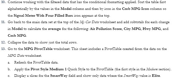
10. Continue working with the filtered date that has the conditional formatting applied. Sort the table first alphabetically by the values in the Model column and then by icon in the Cmb MPG Icon column so the Signal Meter With Four Filled Bars icon appears at the top. 11. Go back to the main data set at the top of the My Car Date worksheet and add subtotals for each change in Model to calculate the average for the following: Air Pollution Score, City MPG, Hwy MPG, and Cmb MPG. 12. Collapse the data to show just the total rows. 13. Go to the MPG PivotTable worksheet. This sheet includes a PivotTable created from the data on the MPG Data worksheet. a. Refresh the PivotTable data. b. Apply the Pivot Style Medium 1 Quick Style to the PivotTable (the first style in the Medhow section). c. Display a slicer for the SmartWay field and show only data where the SwartWay value is Elite