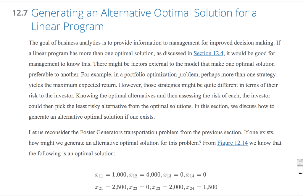
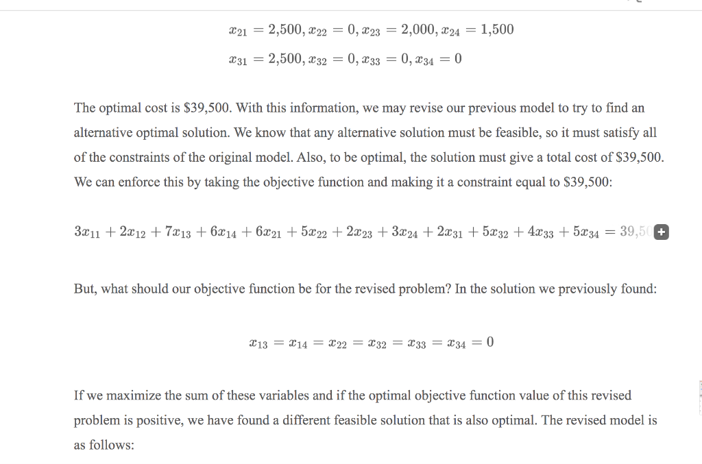
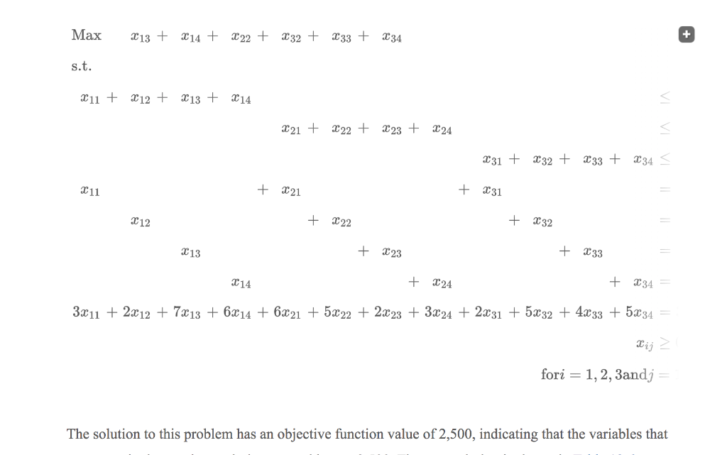
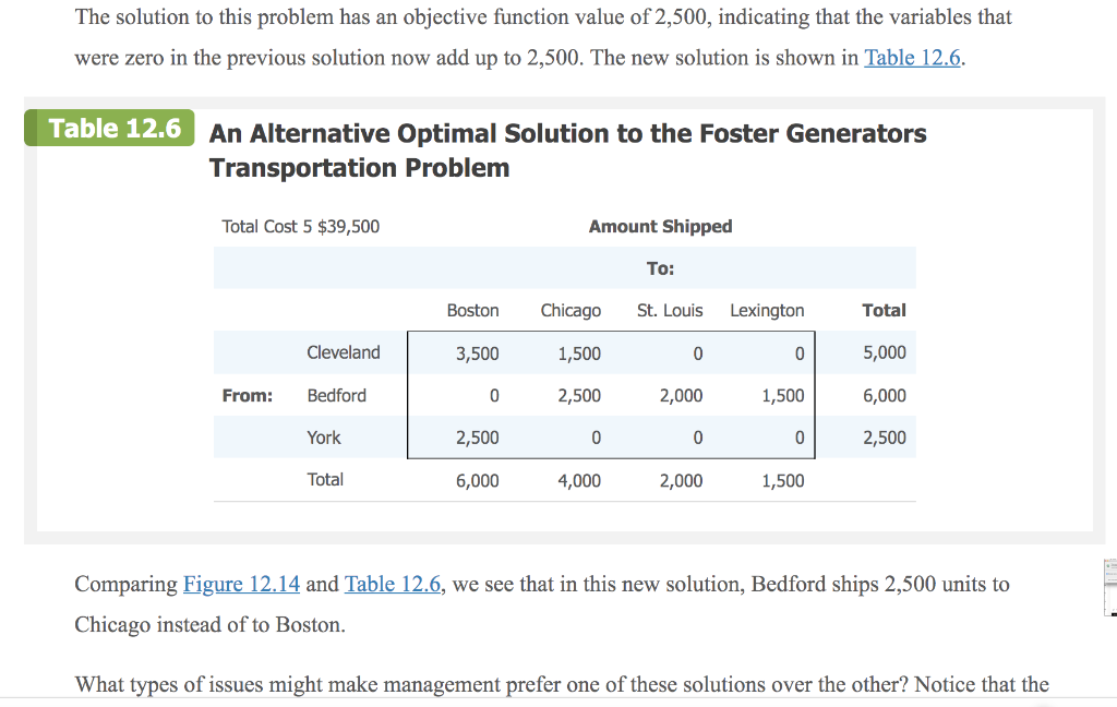
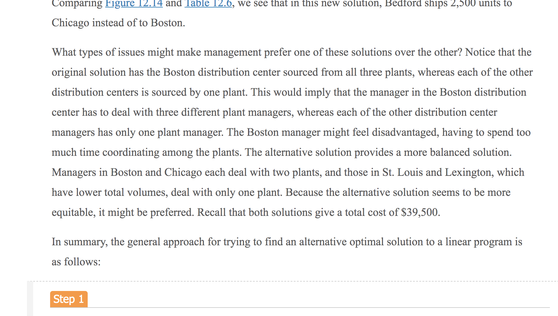
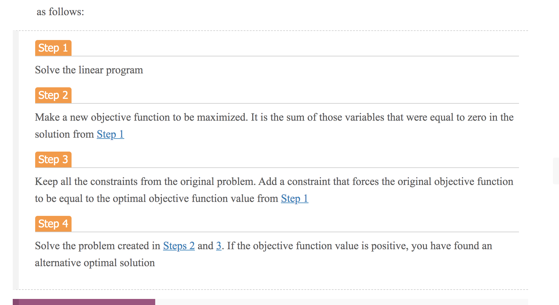
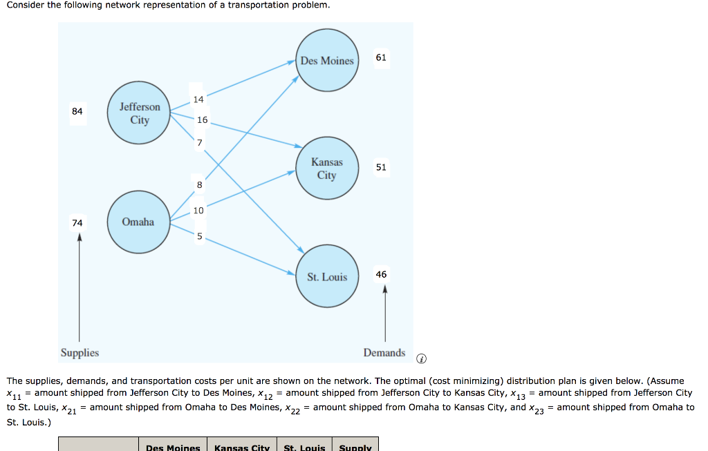
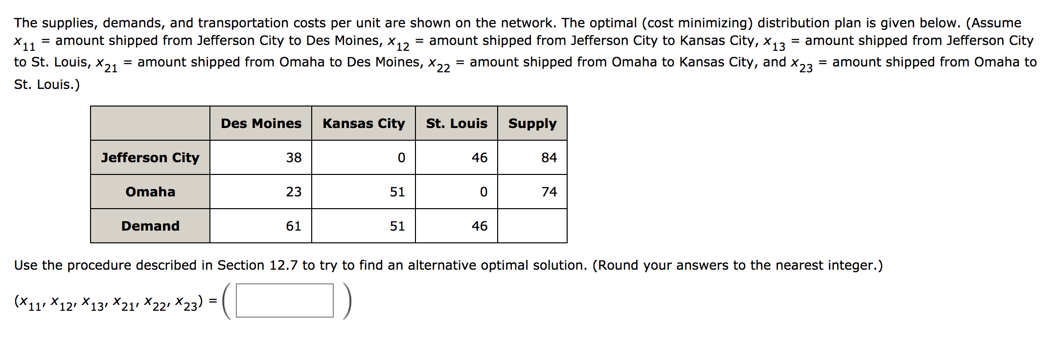
12.7 Generating an Alternative Optimal Solution for a Linear Program The goal of business analytics is to provide information to management for improved decision making. If a linear program has more than one optimal solution, as discussed in Section 12.4, it would be good for management to know this. There might be factors external to the model that make one optimal solution preferable to another. For example, in a portfolio optimization problem, perhaps more than one strategy yields the maximum expected return. However, those strategies might be quite different in terms of their risk to the investor. Knowing the optimal alternatives and then assessing the risk of each, the investor could then pick the least risky alternative from the optimal solutions. In this section, we discuss how to generate an alternative optimal solution if one exists. Let us reconsider the Foster Generators transportation problem from the previous section. If one exists, how might we generate an alternative optimal solution for this problem? From Figure 12.14 we know that the following is an optimal solution: 311 = 1,000, 212 = 4,000, X13 = 0, X14 = 0 X21 = 2,500, 222 = 0, 223 = 2,000, C24 = 1,500 X21 = 2,500, 222 = 0, X23 = 2,000, X24 = 1,500 X31 = 2,500, 232 = 0, 333 = 0, $34 = 0 The optimal cost is $39,500. With this information, we may revise our previous model to try to find an alternative optimal solution. We know that any alternative solution must be feasible, so it must satisfy all of the constraints of the original model. Also, to be optimal, the solution must give a total cost of $39,500. We can enforce this by taking the objective function and making it a constraint equal to $39,500: 3.211 + 2:12 + 7213 + 6214 +6221 + 5222 + 2.623 + 3.224 +2.231 + 5*32 + 4x33 + 5.334 = 39,5 + But, what should our objective function be for the revised problem? In the solution we previously found: 213 = 214 = 222 = 232 = 233 = 234 = 0 If we maximize the sum of these variables and if the optimal objective function value of this revised problem is positive, we have found a different feasible solution that is also optimal. The revised model is as follows: Max 213 + 14 + 222 + 232 + 233 + 234 + s.t. 211 + 12 + 213 + 14 VIVI 821 + 222 + 223 + 224 231 + 32 + 233 + 234 LA 211 + 221 + 231 12 + 222 + 332 213 + 123 + 233 314 + 224 + 234 3x11 + 2x12 + 7x13 + 6x14 + 6x21 + 5X22 + 2x23 + 3.224 + 2x31 + 5X32 + 4x 33 + 5334 Dij fori = 1, 2, 3andy The solution to this problem has an objective function value of 2,500, indicating that the variables that The solution to this problem has an objective function value of 2,500, indicating that the variables that were zero in the previous solution now add up to 2,500. The new solution is shown in Table 12.6. Table 12.6 An Alternative Optimal Solution to the Foster Generators Transportation Problem Total Cost 5 $39,500 Amount Shipped To: Boston Chicago St. Louis Lexington Total Cleveland 3,500 1,500 0 0 5,000 From: Bedford 0 2,500 2,000 1,500 6,000 York 2,500 0 0 0 2,500 Total 6,000 4,000 2,000 1,500 Comparing Figure 12.14 and Table 12.6, we see that in this new solution, Bedford ships 2,500 units to Chicago instead of to Boston. What types of issues might make management prefer one of these solutions over the other? Notice that the Comparing Figure 12.14 and Table 12.6, we see that in this new solution, Bedford ships 2,500 units to Chicago instead of to Boston. What types of issues might make management prefer one of these solutions over the other? Notice that the original solution has the Boston distribution center sourced from all three plants, whereas each of the other distribution centers sourced by one plant. This would imply that the manager in the Boston distribution center has to deal with three different plant managers, whereas each of the other distribution center managers has only one plant manager. The Boston manager might feel disadvantaged, having to spend too much time coordinating among the plants. The alternative solution provides a more balanced solution. Managers in Boston and Chicago each deal with two plants, and those in St. Louis and Lexington, which have lower total volumes, deal with only one plant. Because the alternative solution seems to be more equitable, it might be preferred. Recall that both solutions give a total cost of $39,500. In summary, the general approach for trying to find an alternative optimal solution to a linear program is as follows: Step 1 as follows: Step 1 Solve the linear program Step 2 Make a new objective function to be maximized. It is the sum of those variables that were equal to zero in the solution from Step 1 Step 3 Keep all the constraints from the original problem. Add a constraint that forces the original objective function to be equal to the optimal objective function value from Step 1 Step 4 Solve the problem created in Steps 2 and 3. If the objective function value is positive, you have found an alternative optimal solution Consider the following network representation of a transportation problem. Des Moines 61 14 84 Jefferson City 16 7 Kansas City 51 8 10 74 Omaha Omaha 5 St. Louis 46 Supplies Demands The supplies, demands, and transportation costs per unit are shown on the network. The optimal (cost minimizing) distribution plan is given below. (Assume *11 = amount shipped from Jefferson City to Des Moines, X12 = amount shipped from Jefferson City to Kansas City, *13 = amount shipped from Jefferson City to St. Louis, X21 = amount shipped from Omaha to Des Moines, X22 = amount shipped from Omaha to Kansas City, and X23 = amount shipped from Omaha to St. Louis.) Des Moines Kansas City St. Louis Supply The supplies, demands, and transportation costs per unit are shown on the network. The optimal (cost minimizing) distribution plan is given below. (Assume X11 = amount shipped from Jefferson City to Des Moines, x X12 amount shipped from Jefferson City to Kansas City, X13 amount shipped from Jefferson City to St. Louis, X21 = amount shipped from Omaha to Des Moines, X22 = amount shipped from Omaha to Kansas City, and X23 = amount shipped from Omaha to St. Louis.) Des Moines Kansas City St. Louis Supply Jefferson City 38 0 46 84 Omaha 23 51 0 74 Demand 61 51 46 Use the procedure described in Section 12.7 to try to find an alternative optimal solution. (Round your answers to the nearest integer.) (X11, X12, X13, X21, X22, X23) = ) ( 12.7 Generating an Alternative Optimal Solution for a Linear Program The goal of business analytics is to provide information to management for improved decision making. If a linear program has more than one optimal solution, as discussed in Section 12.4, it would be good for management to know this. There might be factors external to the model that make one optimal solution preferable to another. For example, in a portfolio optimization problem, perhaps more than one strategy yields the maximum expected return. However, those strategies might be quite different in terms of their risk to the investor. Knowing the optimal alternatives and then assessing the risk of each, the investor could then pick the least risky alternative from the optimal solutions. In this section, we discuss how to generate an alternative optimal solution if one exists. Let us reconsider the Foster Generators transportation problem from the previous section. If one exists, how might we generate an alternative optimal solution for this problem? From Figure 12.14 we know that the following is an optimal solution: 311 = 1,000, 212 = 4,000, X13 = 0, X14 = 0 X21 = 2,500, 222 = 0, 223 = 2,000, C24 = 1,500 X21 = 2,500, 222 = 0, X23 = 2,000, X24 = 1,500 X31 = 2,500, 232 = 0, 333 = 0, $34 = 0 The optimal cost is $39,500. With this information, we may revise our previous model to try to find an alternative optimal solution. We know that any alternative solution must be feasible, so it must satisfy all of the constraints of the original model. Also, to be optimal, the solution must give a total cost of $39,500. We can enforce this by taking the objective function and making it a constraint equal to $39,500: 3.211 + 2:12 + 7213 + 6214 +6221 + 5222 + 2.623 + 3.224 +2.231 + 5*32 + 4x33 + 5.334 = 39,5 + But, what should our objective function be for the revised problem? In the solution we previously found: 213 = 214 = 222 = 232 = 233 = 234 = 0 If we maximize the sum of these variables and if the optimal objective function value of this revised problem is positive, we have found a different feasible solution that is also optimal. The revised model is as follows: Max 213 + 14 + 222 + 232 + 233 + 234 + s.t. 211 + 12 + 213 + 14 VIVI 821 + 222 + 223 + 224 231 + 32 + 233 + 234 LA 211 + 221 + 231 12 + 222 + 332 213 + 123 + 233 314 + 224 + 234 3x11 + 2x12 + 7x13 + 6x14 + 6x21 + 5X22 + 2x23 + 3.224 + 2x31 + 5X32 + 4x 33 + 5334 Dij fori = 1, 2, 3andy The solution to this problem has an objective function value of 2,500, indicating that the variables that The solution to this problem has an objective function value of 2,500, indicating that the variables that were zero in the previous solution now add up to 2,500. The new solution is shown in Table 12.6. Table 12.6 An Alternative Optimal Solution to the Foster Generators Transportation Problem Total Cost 5 $39,500 Amount Shipped To: Boston Chicago St. Louis Lexington Total Cleveland 3,500 1,500 0 0 5,000 From: Bedford 0 2,500 2,000 1,500 6,000 York 2,500 0 0 0 2,500 Total 6,000 4,000 2,000 1,500 Comparing Figure 12.14 and Table 12.6, we see that in this new solution, Bedford ships 2,500 units to Chicago instead of to Boston. What types of issues might make management prefer one of these solutions over the other? Notice that the Comparing Figure 12.14 and Table 12.6, we see that in this new solution, Bedford ships 2,500 units to Chicago instead of to Boston. What types of issues might make management prefer one of these solutions over the other? Notice that the original solution has the Boston distribution center sourced from all three plants, whereas each of the other distribution centers sourced by one plant. This would imply that the manager in the Boston distribution center has to deal with three different plant managers, whereas each of the other distribution center managers has only one plant manager. The Boston manager might feel disadvantaged, having to spend too much time coordinating among the plants. The alternative solution provides a more balanced solution. Managers in Boston and Chicago each deal with two plants, and those in St. Louis and Lexington, which have lower total volumes, deal with only one plant. Because the alternative solution seems to be more equitable, it might be preferred. Recall that both solutions give a total cost of $39,500. In summary, the general approach for trying to find an alternative optimal solution to a linear program is as follows: Step 1 as follows: Step 1 Solve the linear program Step 2 Make a new objective function to be maximized. It is the sum of those variables that were equal to zero in the solution from Step 1 Step 3 Keep all the constraints from the original problem. Add a constraint that forces the original objective function to be equal to the optimal objective function value from Step 1 Step 4 Solve the problem created in Steps 2 and 3. If the objective function value is positive, you have found an alternative optimal solution Consider the following network representation of a transportation problem. Des Moines 61 14 84 Jefferson City 16 7 Kansas City 51 8 10 74 Omaha Omaha 5 St. Louis 46 Supplies Demands The supplies, demands, and transportation costs per unit are shown on the network. The optimal (cost minimizing) distribution plan is given below. (Assume *11 = amount shipped from Jefferson City to Des Moines, X12 = amount shipped from Jefferson City to Kansas City, *13 = amount shipped from Jefferson City to St. Louis, X21 = amount shipped from Omaha to Des Moines, X22 = amount shipped from Omaha to Kansas City, and X23 = amount shipped from Omaha to St. Louis.) Des Moines Kansas City St. Louis Supply The supplies, demands, and transportation costs per unit are shown on the network. The optimal (cost minimizing) distribution plan is given below. (Assume X11 = amount shipped from Jefferson City to Des Moines, x X12 amount shipped from Jefferson City to Kansas City, X13 amount shipped from Jefferson City to St. Louis, X21 = amount shipped from Omaha to Des Moines, X22 = amount shipped from Omaha to Kansas City, and X23 = amount shipped from Omaha to St. Louis.) Des Moines Kansas City St. Louis Supply Jefferson City 38 0 46 84 Omaha 23 51 0 74 Demand 61 51 46 Use the procedure described in Section 12.7 to try to find an alternative optimal solution. (Round your answers to the nearest integer.) (X11, X12, X13, X21, X22, X23) = ) (