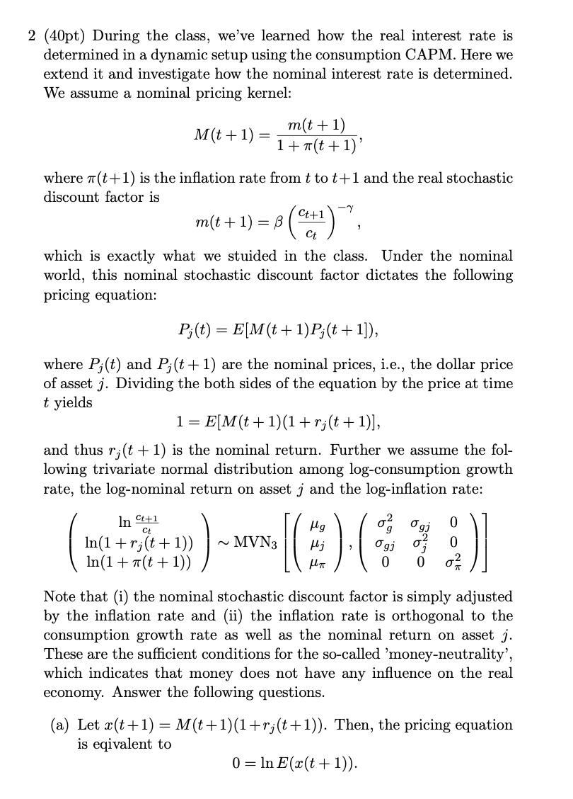
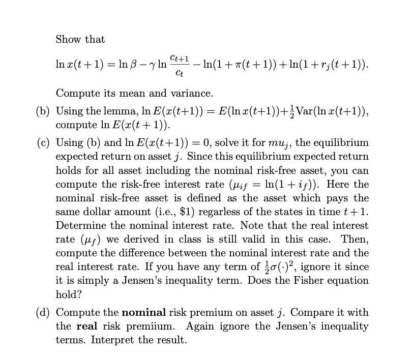
2 (40pt) During the class, we've learned how the real interest rate is determined in a dynamic setup using the consumption CAPM. Here we extend it and investigate how the nominal interest rate is determined. We assume a nominal pricing kernel: M(t+1) m(t+1) 1+#(t + 1)' where #(t+1) is the inflation rate from t to t+1 and the real stochastic discount factor is - Ct+1 m(t + 1) = B Ct which is exactly what we stuided in the class. Under the nominal world, this nominal stochastic discount factor dictates the following pricing equation: P;(t) = E[M(t+1)P;(t+1]), where P;(t) and P;(t+1) are the nominal prices, i.e., the dollar price of asset j. Dividing the both sides of the equation by the price at time t yields 1 = E[M(t+1)(1+ri(t+1)], and thus ri(t+1) is the nominal return. Further we assume the fol- lowing trivariate normal distribution among log-consumption growth rate, the log-nominal return on asset j and the log-inflation rate: In C++1 o Ogj 0 ~MVN3 In(1+r;(t+1)) In(1 + 7 (t + 1)) pg Hj Ogi 0 02 Note that (i) the nominal stochastic discount factor is simply adjusted by the inflation rate and (ii) the inflation rate is orthogonal to the consumption growth rate as well as the nominal return on asset j. These are the sufficient conditions for the so-called 'money-neutrality', which indicates that money does not have any influence on the real economy. Answer the following questions. (a) Let (t+1) = M(t+1)(1+r;(t+1)). Then, the pricing equation is eqivalent to 0 = ln E(2(t+1)). Show that Ct+1 In x(t+1) = In B y In In(1+7(t+1)] +In(1+r;(t+1)). Ct Compute its mean and variance. (b) Using the lemma, In E(x(t+1)) = E(In x(t+1))+ Var(In (t+1)), compute In E(x(t + 1)). (c) Using (b) and in E(x(t+1)) = 0, solve it for muj, the equilibrium expected return on asset j. Since this equilibrium expected return holds for all asset including the nominal risk-free asset, you can compute the risk-free interest rate (Mif = ln(1 + if)). Here the nominal risk-free asset is defined as the asset which pays the same dollar amount (i.e., $1) regarless of the states in time t+1. Determine the nominal interest rate. Note that the real interest rate (uf) we derived in class is still valid in this case. Then, compute the difference between the nominal interest rate and the real interest rate. If you have any term of o(.)?, ignore it since it is simply a Jensen's inequality term. Does the Fisher equation hold? (d) Compute the nominal risk premium on asset j. Compare it with the real risk premiium. Again ignore the Jensen's inequality terms. Interpret the result. 2 (40pt) During the class, we've learned how the real interest rate is determined in a dynamic setup using the consumption CAPM. Here we extend it and investigate how the nominal interest rate is determined. We assume a nominal pricing kernel: M(t+1) m(t+1) 1+#(t + 1)' where #(t+1) is the inflation rate from t to t+1 and the real stochastic discount factor is - Ct+1 m(t + 1) = B Ct which is exactly what we stuided in the class. Under the nominal world, this nominal stochastic discount factor dictates the following pricing equation: P;(t) = E[M(t+1)P;(t+1]), where P;(t) and P;(t+1) are the nominal prices, i.e., the dollar price of asset j. Dividing the both sides of the equation by the price at time t yields 1 = E[M(t+1)(1+ri(t+1)], and thus ri(t+1) is the nominal return. Further we assume the fol- lowing trivariate normal distribution among log-consumption growth rate, the log-nominal return on asset j and the log-inflation rate: In C++1 o Ogj 0 ~MVN3 In(1+r;(t+1)) In(1 + 7 (t + 1)) pg Hj Ogi 0 02 Note that (i) the nominal stochastic discount factor is simply adjusted by the inflation rate and (ii) the inflation rate is orthogonal to the consumption growth rate as well as the nominal return on asset j. These are the sufficient conditions for the so-called 'money-neutrality', which indicates that money does not have any influence on the real economy. Answer the following questions. (a) Let (t+1) = M(t+1)(1+r;(t+1)). Then, the pricing equation is eqivalent to 0 = ln E(2(t+1)). Show that Ct+1 In x(t+1) = In B y In In(1+7(t+1)] +In(1+r;(t+1)). Ct Compute its mean and variance. (b) Using the lemma, In E(x(t+1)) = E(In x(t+1))+ Var(In (t+1)), compute In E(x(t + 1)). (c) Using (b) and in E(x(t+1)) = 0, solve it for muj, the equilibrium expected return on asset j. Since this equilibrium expected return holds for all asset including the nominal risk-free asset, you can compute the risk-free interest rate (Mif = ln(1 + if)). Here the nominal risk-free asset is defined as the asset which pays the same dollar amount (i.e., $1) regarless of the states in time t+1. Determine the nominal interest rate. Note that the real interest rate (uf) we derived in class is still valid in this case. Then, compute the difference between the nominal interest rate and the real interest rate. If you have any term of o(.)?, ignore it since it is simply a Jensen's inequality term. Does the Fisher equation hold? (d) Compute the nominal risk premium on asset j. Compare it with the real risk premiium. Again ignore the Jensen's inequality terms. Interpret the result