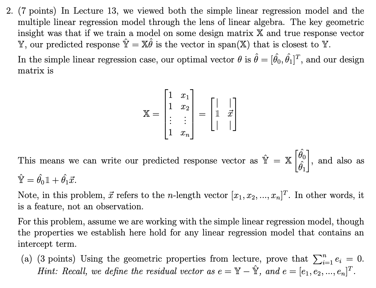
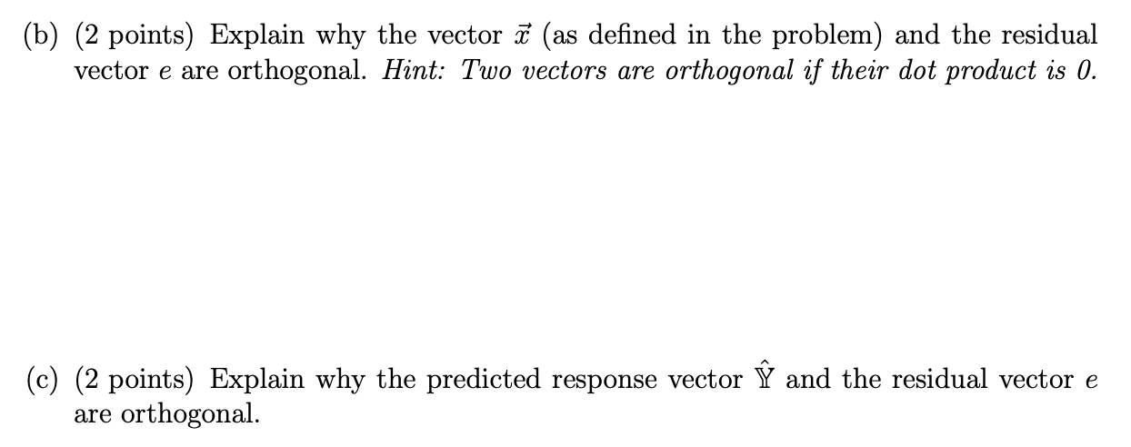
2. (7 points) In Lecture 13, we viewed both the simple linear regression model and the multiple linear regression model through the lens of linear algebra. The key geometric insight was that if we train a model on some design matrix X and true response vector if, our predicted response Y: X6 is the vector in span(X) that 1s closest to Y. In the simple linear regression case, our optimal vector 6 1s 6 = [60, 61]T , and our design matrix is || X=_ =1a' ' II This means we can write our predicted response vector as Y2 K [3:0] , and also as 1 A = (5011 + 9153. Note, in this problem, 5? refers to the nlength vector [3:1, 21:2, ..., mn]T. In other words, it is a feature, not an observation. For this problem, assume we are working with the simple linear regression model, though the properties we establish here hold for any linear regression model that contains an intercept term. (a) (3 points) Using the geometric properties from lecture, prove that 2?:161 2 O. Hint: Recall, we dene the residual vector as e = Y Y, and e = [e1, e2, ..., en]T. (b) (2 points) Explain why the vector x (as defined in the problem) and the residual vector e are orthogonal. Hint: Two vectors are orthogonal if their dot product is 0. (c) (2 points) Explain why the predicted response vector Y and the residual vector e are orthogonal