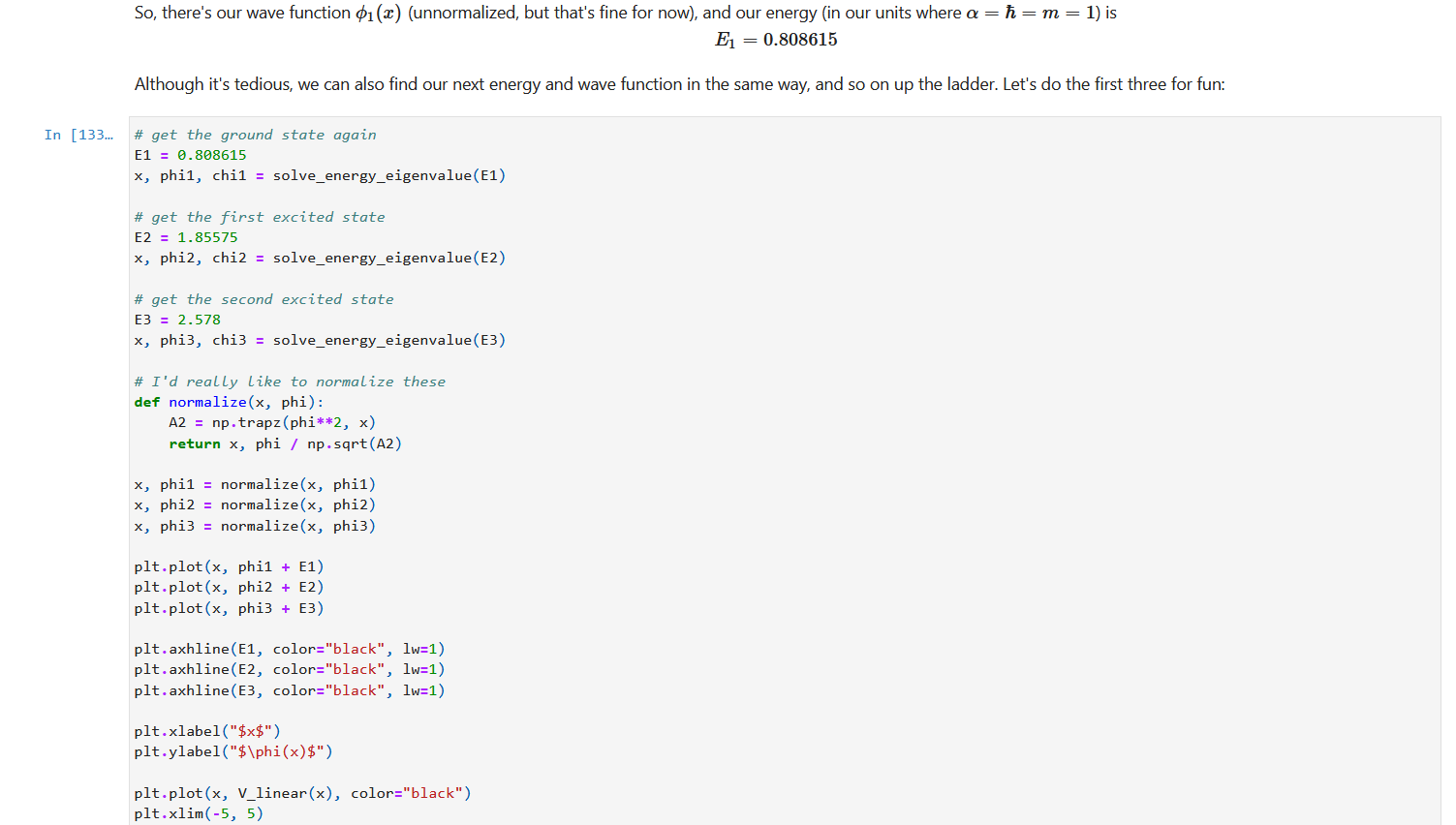
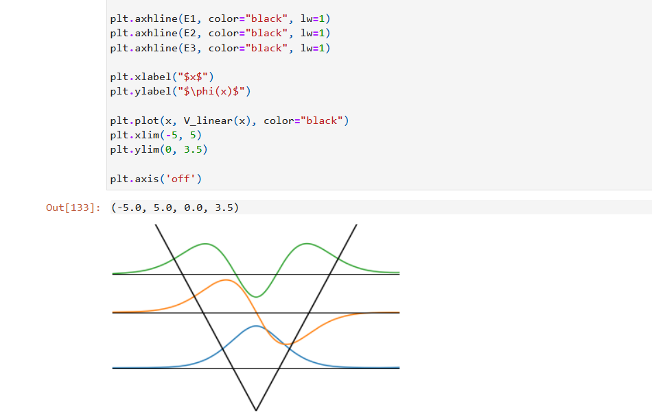
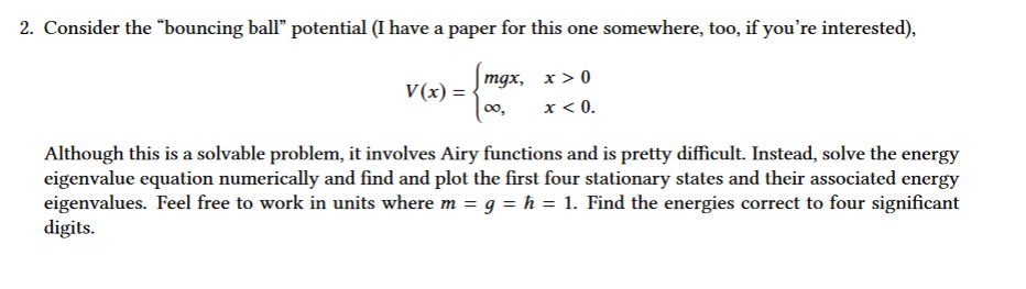
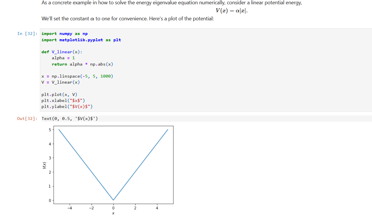
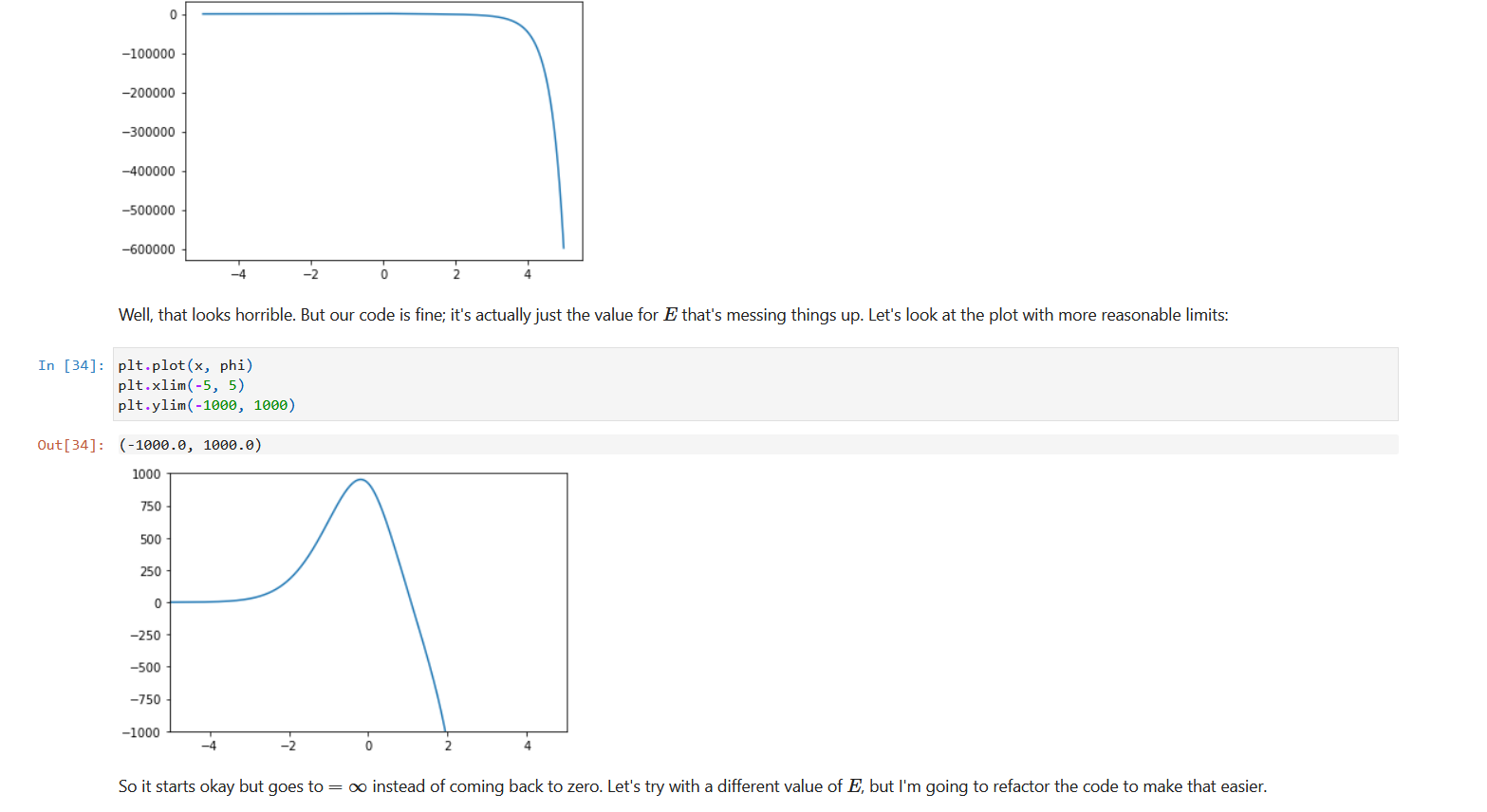
2. Consider the "bouncing ball" potential (I have a paper for this one somewhere, too, if you're interested), mgx, x > 0 V(x) = co , x ]-100000 -200000 -300000 -400000 -500000 -600000 Well, that looks horrible. But our code is fine; it's actually just the value for E that's messing things up. Let's look at the plot with more reasonable limits: In [34]: plt. plot(x, phi) pit.xlim( -5, 5) (0 00OL '0 000T-) : [DE]no 1000 750 500 250 0 -250 -500 -750 -1000 So it starts okay but goes to = co instead of coming back to zero. Let's try with a different value of E, but I'm going to refactor the code to make that easier.So it starts okay but goes to = oo instead of coming back to zero. Let's try with a different value of E, but I'm going to refactor the code to make that easier. In [38]: def solve_energy_eigenvalue(E, x_inf = 5.0, dx = 0.001, phi_0 = 0.0, chi_0 = 1.0, V = V_linear) : x = np . arange (-x_inf, x_inf, dx) N = len(x) phi = np. zeros (N) chi = np. zeros (N) # set the initial conditions phi [0] = phi_0 chi [0] = chi_0 # Loop over x for i in range (N-1) : phi [i+1] = phi[i] + chi[i] * dx chi [i+1] = chi[i] - 2.0 * (E - V(x[i])) * phi[i] * dx return x, phi, chi x, phi, chi = solve_energy_eigenvalue(0.5) plt. plot(x, phi) pit . xlim( -5, 5) pit . ylim(-1000, 1000) (0 0OOT '0 0901-) : [8E]no 1000 750 500 250 0 -250 -500Oh no, now we have the opposite problem - the wave function is going to too! Luckily, that means that correct value of E is between 0.5 and 1.0. So let's try a few more: In [39]: x, phi, chi = solve_energy_eigenvalue(0.8) pit. plot(x, phi) plt.xlim( -5, 5) pit .ylim(-1000, 1000) (0 0OOT '0 0001-) : [6E]no 1000 750 500 250 0 -250 -500 -750 -1000 N- Still blowing up! In [77]: x, phi, chi = solve_energy_eigenvalue(0.9) plt . plot(x, phi) plt . xlim( -5, 5) plt . ylim( -1000, 1000) Out [77]: (-1000.0, 1000.0)Out [77 ] : (-1000.0, 1000.0) 1000 750 500 250 0 -250 -500 -750 -1000 So now we know the correct value is between 0.8 and 0.9. Some more trial and error can get us the correct value to our desired precision (whatever that may be). In [80]: x, phi, chi = solve_energy_eigenvalue(0. 808615) plt . plot(x, phi) plt . xlim( -5, 5) plt .ylim(-200, 1750) Out [80] : (-200.0, 1750.0) 1750 1500 1250 1000 750 500 250 0So, there's our wave function 1 () (unnormalized, but that's fine for now), and our energy (in our units where a = h = m = 1) is E1 = 0.808615 Although it's tedious, we can also find our next energy and wave function in the same way, and so on up the ladder. Let's do the first three for fun: In [133... # get the ground state again E1 = 0. 808615 x, phil, chil = solve_energy_eigenvalue(E1) # get the first excited state E2 = 1.85575 x, phi2, chi2 = solve_energy_eigenvalue(E2) # get the second excited state E3 = 2.578 x, phi3, chi3 = solve_energy_eigenvalue(E3) # I'd really Like to normalize these def normalize(x, phi) : A2 = np. trapz(phi**2, x) return x, phi / np . sqrt(A2) x, phil = normalize(x, phil) x, phi2 = normalize(x, phi2) x, phi3 = normalize(x, phi3) pit . plot(x, phil + E1) pit . plot(x, phi2 + E2) pit. plot(x, phi3 + E3) pit . axhline(E1, color="black", 1w=1) pit. axhline(E2, color="black", 1w=1) pit . axhline(E3, color="black", 1w=1) pit. xlabel("$x$") pit. ylabel("$\\phi(x)$") pit. plot(x, V_linear(x), color="black") plt. xlim( -5, 5)pit . axhline(E1, color="black", 1w=1) plt . axhline(E2, color="black", 1w=1) plt. axhline(E3, color="black", 1w=1) plt . xlabel("$x$") plt . ylabel("$\\phi(x)$") plt. plot(x, V_linear(x), color="black") plt . xlim( -5, 5) plt .ylim(0, 3.5) plt . axis('off' ) Out [133]: (-5.0, 5.0, 0.0, 3.5)