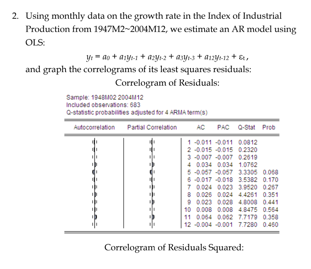
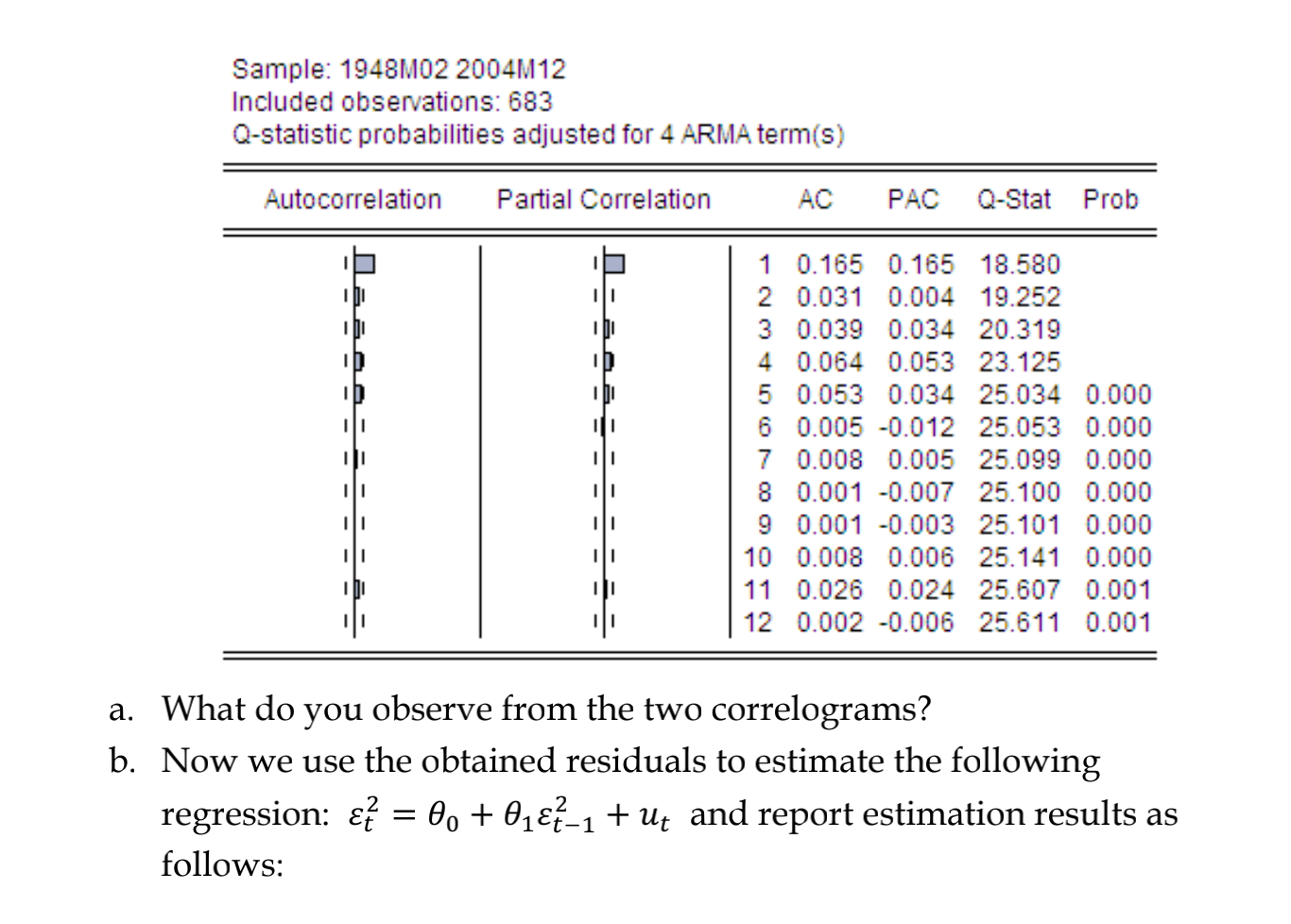
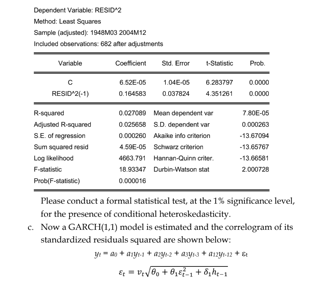
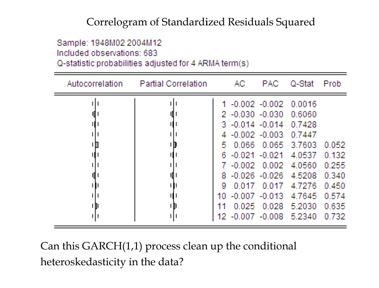
2. Using monthly data on the growth rate in the Index of Industrial Production from 1947M22004M12, we estimate an AR model using OLS: yt = 10 + A1Yt-1 + A2Yt-2 + azyt-3 + 012Yt-12 + Et, + and graph the correlograms of its least squares residuals: Correlogram of Residuals: = Sample: 1948M02 2004M12 Included observations: 683 Q-statistic probabilities adjusted for 4 ARMA term(s) Autocorrelation Partial Correlation AC PAC Q-Stat Prob 111 011 11 11 go 111 1 -0.011 -0.011 0.0812 2 -0.015 -0.015 0.2320 3 -0.007 -0.007 0.2619 4 0.034 0.034 1.0762 5 -0.057 -0.057 3.3305 0.068 6 -0.017 -0.018 3.5382 0.170 7 0.024 0.023 3.9520 0.267 8 0.026 0.024 4.4261 0.351 9 0.023 0.028 4.8008 0.441 10 0.008 0.008 4.8475 0.564 11 0.064 0.062 7.7179 0.358 12 -0.004 -0.001 7.7280 0.460 11 10 Correlogram of Residuals Squared: Sample: 1948M02 2004M12 Included observations: 683 Q-statistic probabilities adjusted for 4 ARMA term(s) Autocorrelation Partial Correlation AC PAC Q-Stat Prob 11 1 0.165 0.165 18.580 2 0.031 0.004 19.252 3 0.039 0.034 20.319 4 0.064 0.053 23.125 5 0.053 0.034 25.034 0.000 6 0.005 -0.012 25.053 0.000 7 0.008 0.005 25.099 0.000 8 0.001 -0.007 25.100 0.000 9 0.001 -0.003 25.101 0.000 10 0.008 0.006 25.141 0.000 11 0.026 0.024 25.607 0.001 12 0.002 -0.006 25.611 0.001 II a. What do you observe from the two correlograms? b. Now we use the obtained residuals to estimate the following regression: &t = 0, + 0182-1 + Ut and report estimation results as follows: = Dependent Variable: RESID^2 Method: Least Squares Sample (adjusted): 1948M03 2004M12 Included observations: 682 after adjustments Variable Coefficient Std. Error t-Statistic Prob. 6.52E-05 1.04E-05 6.283797 0.0000 RESID^2(-1) 0.164583 0.037824 4.351261 0.0000 0.027089 7.80E-05 Mean dependent var S.D. dependent var 0.025658 0.000263 0.000260 Akaike info criterion -13.67094 R-squared Adjusted R-squared S.E. of regression Sum squared resid Log likelihood F-statistic 4.59E-05 Schwarz criterion -13.65767 4663.791 Hannan-Quinn criter. -13.66581 18.93347 Durbin-Watson stat 2.000728 Prob(F-statistic) 0.000016 a Please conduct a formal statistical test, at the 1% significance level, for the presence of conditional heteroskedasticity. c. Now a GARCH(1,1) model is estimated and the correlogram of its standardized residuals squared are shown below: yt = ao + a1yt-1 + a2yt-2 + a3yt-3 + 412Yt-12 + t Et = vtv6, + 017-1 + diht-1 0 : Correlogram of Standardized Residuals Squared Sample: 1948M02 2004M12 Included observations: 683 Q-statistic probabilities adjusted for 4 ARMA term(s) Autocorrelation Partial Correlation AC PAC Q-Stat Prob 11 [1 II 10 II 10 ID 011 1 -0.002 -0.002 0.0016 2 -0.030 -0.030 0.6060 3 -0.014 -0.014 0.7428 4 -0.002 -0.003 0.7447 5 0.066 0.065 3.7603 0.052 6 -0.021 -0.021 4.0537 0.132 7 -0.002 0.002 4.0560 0.255 8 -0.026 -0.026 4.5208 0.340 9 0.017 0.017 4.7276 0.450 10 -0.007 -0.013 4.7645 0.574 11 0.025 0.028 5.2030 0.635 12 -0.007 -0.008 5.2340 0.732 11 010 11 11 11 II Can this GARCH(1,1) process clean up the conditional heteroskedasticity in the data? 2. Using monthly data on the growth rate in the Index of Industrial Production from 1947M22004M12, we estimate an AR model using OLS: yt = 10 + A1Yt-1 + A2Yt-2 + azyt-3 + 012Yt-12 + Et, + and graph the correlograms of its least squares residuals: Correlogram of Residuals: = Sample: 1948M02 2004M12 Included observations: 683 Q-statistic probabilities adjusted for 4 ARMA term(s) Autocorrelation Partial Correlation AC PAC Q-Stat Prob 111 011 11 11 go 111 1 -0.011 -0.011 0.0812 2 -0.015 -0.015 0.2320 3 -0.007 -0.007 0.2619 4 0.034 0.034 1.0762 5 -0.057 -0.057 3.3305 0.068 6 -0.017 -0.018 3.5382 0.170 7 0.024 0.023 3.9520 0.267 8 0.026 0.024 4.4261 0.351 9 0.023 0.028 4.8008 0.441 10 0.008 0.008 4.8475 0.564 11 0.064 0.062 7.7179 0.358 12 -0.004 -0.001 7.7280 0.460 11 10 Correlogram of Residuals Squared: Sample: 1948M02 2004M12 Included observations: 683 Q-statistic probabilities adjusted for 4 ARMA term(s) Autocorrelation Partial Correlation AC PAC Q-Stat Prob 11 1 0.165 0.165 18.580 2 0.031 0.004 19.252 3 0.039 0.034 20.319 4 0.064 0.053 23.125 5 0.053 0.034 25.034 0.000 6 0.005 -0.012 25.053 0.000 7 0.008 0.005 25.099 0.000 8 0.001 -0.007 25.100 0.000 9 0.001 -0.003 25.101 0.000 10 0.008 0.006 25.141 0.000 11 0.026 0.024 25.607 0.001 12 0.002 -0.006 25.611 0.001 II a. What do you observe from the two correlograms? b. Now we use the obtained residuals to estimate the following regression: &t = 0, + 0182-1 + Ut and report estimation results as follows: = Dependent Variable: RESID^2 Method: Least Squares Sample (adjusted): 1948M03 2004M12 Included observations: 682 after adjustments Variable Coefficient Std. Error t-Statistic Prob. 6.52E-05 1.04E-05 6.283797 0.0000 RESID^2(-1) 0.164583 0.037824 4.351261 0.0000 0.027089 7.80E-05 Mean dependent var S.D. dependent var 0.025658 0.000263 0.000260 Akaike info criterion -13.67094 R-squared Adjusted R-squared S.E. of regression Sum squared resid Log likelihood F-statistic 4.59E-05 Schwarz criterion -13.65767 4663.791 Hannan-Quinn criter. -13.66581 18.93347 Durbin-Watson stat 2.000728 Prob(F-statistic) 0.000016 a Please conduct a formal statistical test, at the 1% significance level, for the presence of conditional heteroskedasticity. c. Now a GARCH(1,1) model is estimated and the correlogram of its standardized residuals squared are shown below: yt = ao + a1yt-1 + a2yt-2 + a3yt-3 + 412Yt-12 + t Et = vtv6, + 017-1 + diht-1 0 : Correlogram of Standardized Residuals Squared Sample: 1948M02 2004M12 Included observations: 683 Q-statistic probabilities adjusted for 4 ARMA term(s) Autocorrelation Partial Correlation AC PAC Q-Stat Prob 11 [1 II 10 II 10 ID 011 1 -0.002 -0.002 0.0016 2 -0.030 -0.030 0.6060 3 -0.014 -0.014 0.7428 4 -0.002 -0.003 0.7447 5 0.066 0.065 3.7603 0.052 6 -0.021 -0.021 4.0537 0.132 7 -0.002 0.002 4.0560 0.255 8 -0.026 -0.026 4.5208 0.340 9 0.017 0.017 4.7276 0.450 10 -0.007 -0.013 4.7645 0.574 11 0.025 0.028 5.2030 0.635 12 -0.007 -0.008 5.2340 0.732 11 010 11 11 11 II Can this GARCH(1,1) process clean up the conditional heteroskedasticity in the data