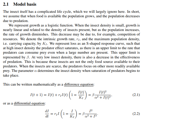
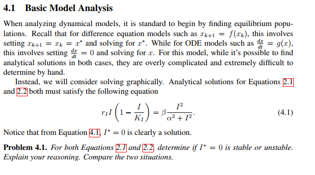
2.1 Model basis The insect itself has a complicated life cycle, which we will largely ignore here. In short, we assume that when food is available the population grows, and the population decreases due to predation. We represent growth as a logistic function. 1|When the insect density is small, growth is nearly linear and related to the density of insects present, but as the population increases, the rate of growth diminishes. This decrease may be due to, for example, competition of resources. We denote the intrinsic growth rate, n, and the maximum population density, i.e. carrying capacity, by K;. We represent loss as an Sshaped response curve, such that at high insect density the predator effect saturates, as there is an upper limit to the rate that predators can consume prey even when a large number are present. This upper limit is represented by ,5. At very low insect density, there is also a decrease in the effectiveness of predation. This is because these insects are not the only food source available to their predators. When the insects are scarce, the predators focus on other more readily available prey. The parameter 11 determines the insect density when saturation of predators begins to take place. This can be written mathematically as a di'erence guation: I[t+1)=I{t)+ryI[t]( %) $m (2.1) or as a differential guaon: d! I F 521']! (1?!) 2+I2. [2.2) 4.1 Basic Model Analysis When analyzing dynamical models, it is standard to begin by finding equilibrium popu- lations. Recall that for difference equation models such as The1 = f(I), this involves setting Tel = T = c* and solving for r*. While for ODE models such as " = g(x), this involves setting d = 0 and solving for x. For this model, while it's possible to find analytical solutions in both cases, they are overly complicated and extremely difficult to determine by hand. Instead, we will consider solving graphically. Analytical solutions for Equations 2.I and 2.2 both must satisfy the following equation m 1 - = 3 (4.1) KI Notice that from Equation 4.1 /* = 0 is clearly a solution. Problem 4.1. For both Equations 2.] and 2.2 determine if I* = 0 is stable or unstable. Explain your reasoning. Compare the two situations