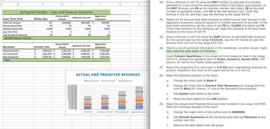
23. Enter a formula in cell C9 using the PMT function to calculate the monthly payment on a loan using the assumptions listed in the Status Quo scenario. In the PMT formula, use C6 as the monthly interest rate (rate), C8 as the total number of payments (nper), and C4 as the loan amount (pv). Enter this formula in cell C9, and then copy the formula to the range 09:F9. Growth Moderate Growth gressive Expansion SpringLeaf Designs - Loan and Revenue Scenarios Conservative Loan Term (Yrs) Status Que Growth Total Loan Amount $150,000 S350,000 Annual interest Rate Monthly interest Rate 0.40 0.40% Loan Term (Yrs) Total Number of Payments Monthly Payment Amount 0.40% 24. Select cell F9 and use Goal Seek Analysis to determine the loan amount in the Aggressive Expansion scenario based on a monthly payment of $12,000. In the Goal Seek calculations, set the value of cell F9 to -12,000 and select cell F4 (Total Loan Amount) as the changing cell. Keep the outcome of the Goal Seek Analysis as the value of cell F4. 25. Enter a formula in cell C15 using the SUM function to calculate total revenues for the current year (or the range C12:C14). Use the Fill Handle to copy the formula from cell C15 to the range D15:F15 26. There's a lot of numerical information in this worksheet, so some visuals might help make the data easier to interpret. Conservative Revenues Current Year Aggressive Expansion Growth Moderate Growth 4 Head Accessories Arm Accessories Body Accessories 3,047,520 S 3,591,816 $ 5,289,720 $ 3152,272 S 950,998 5.818,692 $ $ ,266,528 $ 5,028,542 $ 7,405,608 $ 5,333,160 6.285.678 9.257,010 $ Insert Column Sparklines in the range G12:G14 based on data in the range C12:F14. Change the sparkline color to Green, Accent 6, Darker 50% (10th column, 6th row of the Theme Colors palette). 27. Select the range B12:C14, and insert a 2-D Pie chart segmenting revenues by product. Reposition the chart so the upper left corner is in cell H2. 28. Make the following changes to the chart: a. Change the chart style to Style 2 b. Change the chart title to Current Year Revenues and change the font color to Blue (8th column, 1 row of the Standard Colors palette). ACTUAL AND PROJECTED REVENUES Head Arm o r Body Accessories 59.257.000 SSL $5.333,16 C. Add Center data labels to the chart. d. Move the chart legend to the Left position 29. Select the Actual and Projected Revenues chart located in the range H16:M30. Make the following changes to the chart: a. Change the major units of the vertical axis to 5000000 b. Add Growth Scenarios as the horizontal axis title and Revenue as the vertical axis title. c. Remove the data labels from the graph. Current Consive Growth Mod Growth Acressive 23. Enter a formula in cell C9 using the PMT function to calculate the monthly payment on a loan using the assumptions listed in the Status Quo scenario. In the PMT formula, use C6 as the monthly interest rate (rate), C8 as the total number of payments (nper), and C4 as the loan amount (pv). Enter this formula in cell C9, and then copy the formula to the range 09:F9. Growth Moderate Growth gressive Expansion SpringLeaf Designs - Loan and Revenue Scenarios Conservative Loan Term (Yrs) Status Que Growth Total Loan Amount $150,000 S350,000 Annual interest Rate Monthly interest Rate 0.40 0.40% Loan Term (Yrs) Total Number of Payments Monthly Payment Amount 0.40% 24. Select cell F9 and use Goal Seek Analysis to determine the loan amount in the Aggressive Expansion scenario based on a monthly payment of $12,000. In the Goal Seek calculations, set the value of cell F9 to -12,000 and select cell F4 (Total Loan Amount) as the changing cell. Keep the outcome of the Goal Seek Analysis as the value of cell F4. 25. Enter a formula in cell C15 using the SUM function to calculate total revenues for the current year (or the range C12:C14). Use the Fill Handle to copy the formula from cell C15 to the range D15:F15 26. There's a lot of numerical information in this worksheet, so some visuals might help make the data easier to interpret. Conservative Revenues Current Year Aggressive Expansion Growth Moderate Growth 4 Head Accessories Arm Accessories Body Accessories 3,047,520 S 3,591,816 $ 5,289,720 $ 3152,272 S 950,998 5.818,692 $ $ ,266,528 $ 5,028,542 $ 7,405,608 $ 5,333,160 6.285.678 9.257,010 $ Insert Column Sparklines in the range G12:G14 based on data in the range C12:F14. Change the sparkline color to Green, Accent 6, Darker 50% (10th column, 6th row of the Theme Colors palette). 27. Select the range B12:C14, and insert a 2-D Pie chart segmenting revenues by product. Reposition the chart so the upper left corner is in cell H2. 28. Make the following changes to the chart: a. Change the chart style to Style 2 b. Change the chart title to Current Year Revenues and change the font color to Blue (8th column, 1 row of the Standard Colors palette). ACTUAL AND PROJECTED REVENUES Head Arm o r Body Accessories 59.257.000 SSL $5.333,16 C. Add Center data labels to the chart. d. Move the chart legend to the Left position 29. Select the Actual and Projected Revenues chart located in the range H16:M30. Make the following changes to the chart: a. Change the major units of the vertical axis to 5000000 b. Add Growth Scenarios as the horizontal axis title and Revenue as the vertical axis title. c. Remove the data labels from the graph. Current Consive Growth Mod Growth Acressive