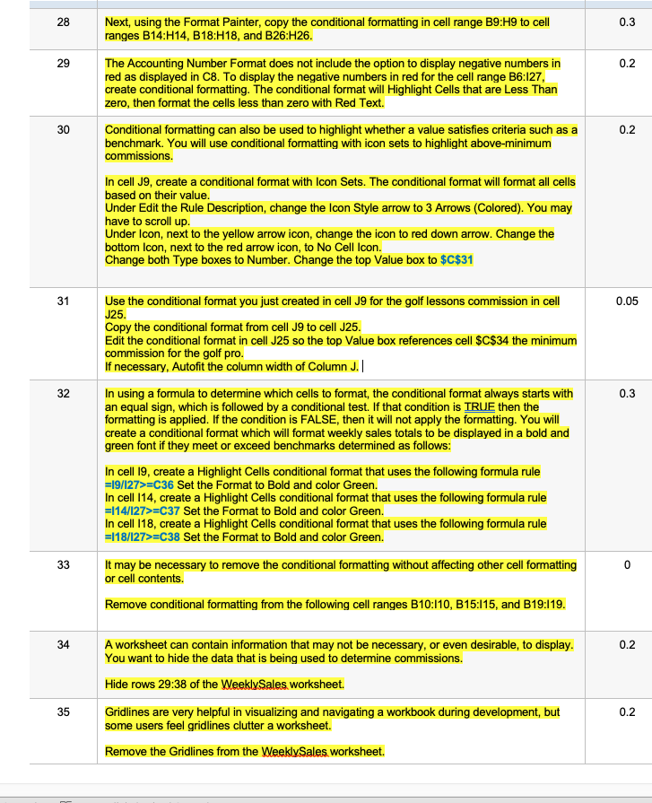
28 0.3 29 0.2 Next, using the Format Painter, copy the conditional formatting in cell range B9:H9 to cell ranges B14:H14, B18:H18, and B26:H26. The Accounting Number Format does not include the option to display negative numbers in red as displayed in C8. To display the negative numbers in red for the cell range B6:127, create conditional formatting. The conditional format will Highlight Cells that are Less Than zero, then format the cells less than zero with Red Text. Conditional formatting can also be used to highlight whether a value satisfies criteria such as a benchmark. You will use conditional formatting with icon sets to highlight above-minimum commissions. 30 0.2 In cell J9, create a conditional format with Icon Sets. The conditional format will format all cells based on their value. Under Edit the Rule Description, change the Icon Style arrow to 3 Arrows (Colored). You may have to scroll up Under Icon, next to the yellow arrow icon, change the icon to red down arrow. Change the bottom Icon, next to the red arrow icon, to No Cell Icon. Change both Type boxes to Number. Change the top Value box to $C$31 31 0.05 32 0.3 Use the conditional format you just created in cell J9 for the golf lessons commission in cell J25. Copy the conditional format from cell J9 to cell J25. Edit the conditional format in cell J25 so the top Value box references cell $C$34 the minimum commission for the golf pro. If necessary, Autofit the column width of Column J.|| In using a formula to determine which cells to format, the conditional format always starts with an equal sign, which is followed by a conditional test. If that condition is TRUE then the formatting is applied. If the condition is FALSE, then it will not apply the formatting. You will create a conditional format which will format weekly sales totals to be displayed in a bold and green font if they meet or exceed benchmarks determined as follows: In cell 19, create a Highlight Cells conditional format that uses the following formula rule =19/127>=C36 Set the Format to Bold and color Green. In cell 114, create a Highlight Cells conditional format that uses the following formula rule =114/127>=C37 Set the Format to Bold and color Green. In cell 118, create a Highlight Cells conditional format that uses the following formula rule =118/127>=C38 Set the Format to Bold and color Green. It may be necessary to remove the conditional formatting without affecting other cell formatting or cell contents. Remove conditional formatting from the following cell ranges B10:110, B15:115, and B19:119. 33 0 34 0.2 A worksheet can contain information that may not be necessary, or even desirable, to display. You want to hide the data that is being used to determine commissions. Hide rows 29:38 of the Weekly Sales, worksheet. Gridlines are very helpful in visualizing and navigating a workbook during development, but some users feel gridlines clutter a worksheet. Remove the Gridlines from the WeeklySales, worksheet. 35 0.2 28 0.3 29 0.2 Next, using the Format Painter, copy the conditional formatting in cell range B9:H9 to cell ranges B14:H14, B18:H18, and B26:H26. The Accounting Number Format does not include the option to display negative numbers in red as displayed in C8. To display the negative numbers in red for the cell range B6:127, create conditional formatting. The conditional format will Highlight Cells that are Less Than zero, then format the cells less than zero with Red Text. Conditional formatting can also be used to highlight whether a value satisfies criteria such as a benchmark. You will use conditional formatting with icon sets to highlight above-minimum commissions. 30 0.2 In cell J9, create a conditional format with Icon Sets. The conditional format will format all cells based on their value. Under Edit the Rule Description, change the Icon Style arrow to 3 Arrows (Colored). You may have to scroll up Under Icon, next to the yellow arrow icon, change the icon to red down arrow. Change the bottom Icon, next to the red arrow icon, to No Cell Icon. Change both Type boxes to Number. Change the top Value box to $C$31 31 0.05 32 0.3 Use the conditional format you just created in cell J9 for the golf lessons commission in cell J25. Copy the conditional format from cell J9 to cell J25. Edit the conditional format in cell J25 so the top Value box references cell $C$34 the minimum commission for the golf pro. If necessary, Autofit the column width of Column J.|| In using a formula to determine which cells to format, the conditional format always starts with an equal sign, which is followed by a conditional test. If that condition is TRUE then the formatting is applied. If the condition is FALSE, then it will not apply the formatting. You will create a conditional format which will format weekly sales totals to be displayed in a bold and green font if they meet or exceed benchmarks determined as follows: In cell 19, create a Highlight Cells conditional format that uses the following formula rule =19/127>=C36 Set the Format to Bold and color Green. In cell 114, create a Highlight Cells conditional format that uses the following formula rule =114/127>=C37 Set the Format to Bold and color Green. In cell 118, create a Highlight Cells conditional format that uses the following formula rule =118/127>=C38 Set the Format to Bold and color Green. It may be necessary to remove the conditional formatting without affecting other cell formatting or cell contents. Remove conditional formatting from the following cell ranges B10:110, B15:115, and B19:119. 33 0 34 0.2 A worksheet can contain information that may not be necessary, or even desirable, to display. You want to hide the data that is being used to determine commissions. Hide rows 29:38 of the Weekly Sales, worksheet. Gridlines are very helpful in visualizing and navigating a workbook during development, but some users feel gridlines clutter a worksheet. Remove the Gridlines from the WeeklySales, worksheet. 35 0.2