# $3$ key statements: numpy, pyplot, inline display

import numpy as np

import matplotlib.pyplot as plt

$\%$matplotlib inline

## Initialization

#Define the function that you're finding the root of

def fn$($x$)$:

return np$.$cos$($x$)$

# Desired error tolerance

tolerance $=1$E$-6$

# No$.$ iterations large enough to guarantee tolerance

maxIt $=100$

#guess for lower and upper bound on root

lower$=1$

upper$=2$

# Create array for error results

maxError $=$ np$.$zeros$($maxIt$+1)$

# Create array for actual error

actualError $=$ np$.$zeros$($maxIt$+1)$

#actual root for cos$($x$)$ between lower and upper $($theoretical$)$

actual $=$ np$.$pi$/2$

#first average to set up first iteration

avg $=($upper$+$lower$)/2$

## Calculation

for i in range$($maxIt$+1)$:

maxError$[$i$]=$upper$-$avg

actualError$[$i$]=$abs$($avg$-$actual$)$

# If tolerance has been met, then exit loop

if maxError$[$itolerance:

break

## Narrow down location of root depending on signs

# First option: if avg is root, then exit loop $($done$)$

if fn$($avg$)==$actual:

break

# Second option: if fn changes sign on left, then move left

elif fn$($lower$)*$fn$($avg$)<mn>0</mn>$:

upper$=$avg

# Last resort: if fn changes sign on right, then move right

else:

lower$=$avg

avg$=($lower$+$upper$)/2$

# Done! Print result

print$("$Estimated root is$",$ avg,"with tolerance", tolerance$)$

## Presentation in a figure

#plot max and actual error versus iteration number

plt$.$figure$(1)$

plt$.$plot$($np$.$arange$($i$+1),$ maxError$[$:i$+1],$ label$=$"Max Error"$)$

plt$.$plot$($np$.$arange$($i$+1),$ actualError$[$:i$+1],$ label$=$"Actual Error"$)$

# Change y scale to logarithmic

plt$.$yscale$(\text{'}$log$\text{'})$

# Add labels to axes

plt$.$xlabel$("$Iteration Number"$)$

plt$.$ylabel$("$Absolute Error"$)$

# Add legend and title.

plt$.$legend$($loc$=2)$

plt$.$title$("$Max and Actual Error for Bisection Method"$)$

plt$.$show$()$

Use this code and change it to match with the following questions:

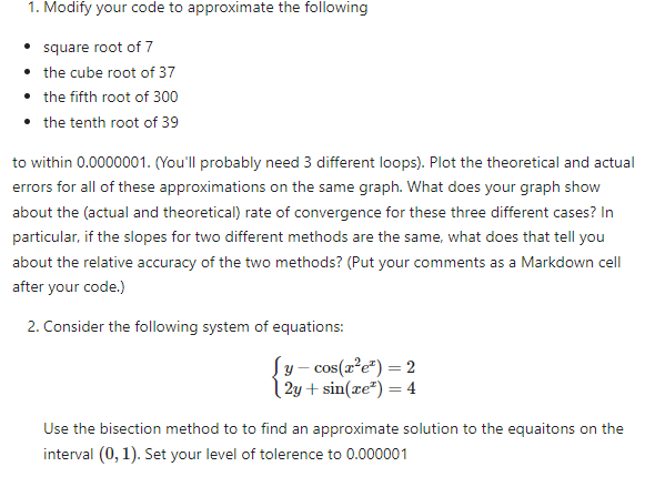
Modify your code to approximate the following

square root of $7$

the cube root of $37$

the fifth root of $300$

the tenth root of $39$

to within $0\mathrm{.}0000001.($You$\text{'}$ll probably need $3$ different loops$).$ Plot the theoretical and actual

errors for all of these approximations on the same graph. What does your graph show

about the $($actual and theoretical$)$ rate of convergence for these three different cases? In

particular, if the slopes for two different methods are the same, what does that tell you

about the relative accuracy of the two methods? $($Put your comments as a Markdown cell

after your code.$)$

Consider the following system of equations:

$y-cos(x^2{e}^x)=2$

$2y+sin(x{e}^x)=4$

Use the bisection method to to find an approximate solution to the equaitons on the

interval $(0,1).$ Set your level of tolerence to $0\mathrm{.}000001$

Use Newton's method to estimate a root of $cosx.$ Initial guess is $2.$

Newton's method equation is:

$x_{i+1}=x_i+\frac{f(x_i)}{f^{\text{'}}(x_i)}$

Relative error equation is

$|lo{n}_a|=|\frac{x_{i+1}-x_i}{x_{i+1}}|100$

Set the max number of iterations for the method at $20$

Set a minimum denominator of $1E-20$

Set a tolerance of $5E-8$ for the relative approximate error