$(3$ pts$)$ You are designing a flow sensor for use with a drug infusion pump. You have a highly accurate bench test to determine the true flow rate for comparison with the flow rate signal output from your sensor$.$ You are changing three of the design parameters in an attempt to minimize the inherent flow rate noise level.

You can run virtual experiments with this system using the spreadsheet provided on Canvas. Using $20$ experimental runs in a CCD design, provide the following:

a$)$ A regression equation for the response surface. $($This surface should be a best fit across the entire allowable range of these design variables.$)$

b$)$ The residuals plot for your response surface.

c$)$ Your proposed optimum settings for the three design variables.

d$)$ A contour plot $($holding one of the variables fixed$)$ that shows the optimum setting point.

$(3$ pts$)$ You want to know an equation to predict the maximum material stress, ${}_{\text{m}\text{a}\text{x}},$ at a specific location of your connecting rod shown to the right. The loading condition is known, but there are two geometric parameters that you can change to affect the maximum stress output. Suppose the FEA model takes $8$ hours to run and you have one week to find the equation for use in subsequent design decisions.

Within a couple days, you are able to use several processor cores on multiple parallel computing clusters to obtain the following max stress values listed at the white square grid points. $($This maximum stress contour surface is actually unknown to you, yet it is shown to make the problem more intuitive. In practice, you would only have the stress values listed at the grid points for which you ran the model.$)$

Given the FEA model results shown at the seven white square grid points, you would like to compute the transfer function model of the following form:

${}_{\text{m}\text{a}\text{x}}=a_0+a_1{x}_1+a_2{x}_2+a_{11}{x}_1^2+a_{22}{x}_2^2+a_{12}{x}_1{x}_2$

You can arrive at such a model using the two$-$dimensional Taylor series expansion about the baseline point $(x_{1B},x_{2BL})$ at the center:

${}_{\text{m}\text{a}\text{x}}={}_{\text{m}\text{a}\text{x}\text{,}BL}+\frac{\text{d}\text{e}\text{l}{}_{\text{m}\text{a}\text{x}}}{del{x}_1}(x_1-x_{1BL})+\frac{\text{d}\text{e}\text{l}{}_{\text{m}\text{a}\text{x}}}{del{x}_2}(x_2-x_{2BL})+(\frac{1}{2})\frac{de{l}^2{}_{\text{m}\text{a}\text{x}}}{del{x}_1^2}(x_1-x_{1BL}{)}^2$

$+(\frac{1}{2})\frac{de{l}^2{}_{\text{m}\text{a}\text{x}}}{del{x}_2^2}(x_2-x_{2BL}{)}^2+\frac{de{l}^2{}_{\text{m}\text{a}\text{x}}}{del{x}_{1}del{x}_2}(x_1-x_{1BL})(x_2-x_{2BL})$

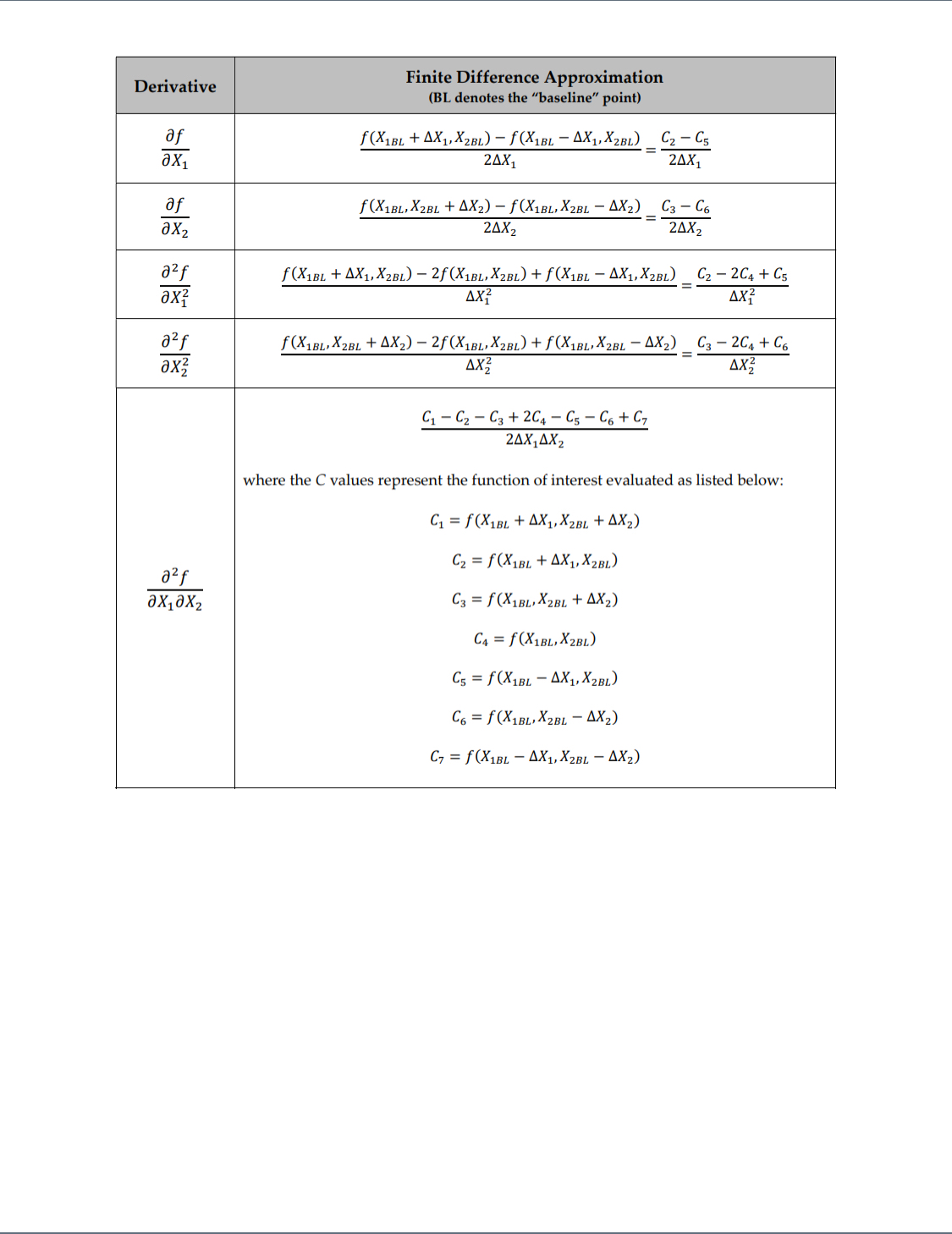
Although this equation looks complex, each of the partial derivatives can be computed from your model output in a straightforward way using a technique called the finite difference approximation. These approximations for a general function $f$ are given in the table on the following page.

Your task is to compute each of the partial derivative approximations in the table from the information provided. You must then fill in Equation $(2)$ with the appropriate numerical values. Simplification of the equation to the form in Equation $(1)$ is not necessary. $($Hint: A spreadsheet is probably the way to go$)$

$\backslash$table$[[$Derivative$,\backslash$table$[[$Finite Difference Approximation$],[($BL denotes the "baseline" point$)]]],[\frac{\text{d}\text{e}\text{l}\text{f}}{del{x}_1},\frac{f(x_{1BL}+x_1,x_{2BL})-f(x_{1BL}-x_1,x_{2BL})}{2x_1}=\frac{C_2-C_5}{2x_1}$