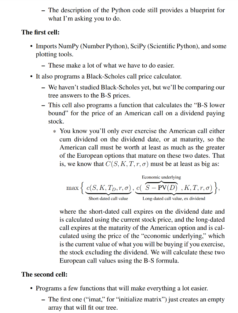
3. Python exercise: Using trees to do real pricing! A note on Python in finance: Industry runs off Python! It is the standard tool used for quantitative finance in the real world, and having some skill with it is incredibly valuable on the job market. Academia uses a lot of Matlab (what I mainly use, for asset pricing and data analysis), Stata (primarily corporate finance researchers using panel data), and SAS (big data sets, especially the trade and quote [or "TAQ," pronounced "tack"] data). With the proper packages Python can do it all, and it's free (a huge plus in industry)! For example, the NumPy package (number python) was basically written to give Python the functionality of Matlab. The big tool used in the finance industry is the PANDAS package (python data analysis), which was written by Wes McKinney while he was working for AQR (Applied Quantitative Research, a large quantitative asset manager in Greenwich, Connecticut). - If you haven't used Python before, want to use the code I provide, and need help getting started, then please start with the "Getting started with Python/Jupyter notebooks' item, on Blackboard before Learning Module 0. Now to the exercise...this is easiest if you start with the Jupyter notebook: "American_Call_Tree_Template_230125.ipynb." This is pre-programmed to do most of the work, and provides a blue-print for the few missing cells (the ones you'll need to fill in to make it work!). You should probably have the note book open and available while going through the following detailed description. - Note: you are not required to do this using Python. - You can use any package you want to (Excel, Matlab, R, Mathematica....whatever you like). - If you want to use something other than Python, however, then you will need to code the whole thing yourself! - The description of the Python code still provides a blueprint for what I'm asking you to do. The first cell: - Imports NumPy (Number Python), SciPy (Scientific Python), and some plotting tools. - These make a lot of what we have to do easier. - It also programs a Black-Scholes call price calculator. - We haven't studied Black-Scholes yet, but we'll be comparing our tree answers to the B-S prices. - This cell also programs a function that calculates the "B-S lower bound" for the price of an American call on a dividend paying stock. * You know you'll only ever exercise the American call either cum dividend on the dividend date, or at maturity, so the American call must be worth at least as much as the greater of the European options that mature on these two dates. That is, we know that C(S,K,T,r,) must be at least as big as: max{Short-datedcallvaluec(S,K,TD,r,),Long-datedcallvalue,exdividendc(SPV(D)Economicunderlying,K,T,r,)}, where the short-dated call expires on the dividend date and is calculated using the current stock price, and the long-dated call expires at the maturity of the American option and is calculated using the price of the "economic underlying," which is the current value of what you will be buying if you exercise, the stock excluding the dividend. We will calculate these two European call values using the B-S formula. The second cell: - Programs a few functions that will make everything a lot easier. - The first one ("imat," for "initialize matrix") just creates an empty array that will fit our tree. - The second one ("maketree") takes the initial stock price (S), the tree primitives (u and d ), and the desired number of steps (n), and returns the corresponding stock price tree. * I gave you this so that you wouldn't have to figure out for yourselves how to make these fairly large NumPy arrays... - The third one ("RNP," for "risk-neutral pricing") takes n+1 payoffs ( PO, an (n+1)1 array, representing the payoffs at the end of an n-periond tree for some asset), together with the riskneutral up-probability (q), and the one-period discount rate (r), and "pulls-back" using the risk-neutral pricing machinery to produce the full n-period price tree for the asset. The third cell: This is the first one that you need to program! You need to program two functions: (a) The first is "CRRTree." - This should have four inputs: a stock's price and volatility ( S and ), together with a time horizon (T) and number of steps (n). - It should calculate the CRR u, and use this in the inputs for the "maketree" function, to produce a tree corresponding to the desired underlying. - It should "return" this tree (i.e., the tree should be the functions output). - My version is just the declaratory statement ("def CRRTree(S,sigma,T,n): and two additional lines. (b) The second is "CRRCall." - This should have six inputs: The five B-S inputs (S,K,T,r, and ), and the number of steps you want to use in your tree (n). - It should create the n-period CRR tree corresponding to your underlying. - It should then calculate the things you need to do the risk-neutral pricing. - The one-period discount rate, given the annualized continuously compounded rate (what you're given in B-S), and hte time-to-maturity and number of steps. - The risk-neutral probability of the up-move on the tree. * In addition to the one-period discount rate, calculating this also requires u and d which you can read right off the stock tree! - The call payoffs at maturity. * These just depend on the stock price at each node in the last step of the tree. - Here I have the declaratory statement and another half dozen lines. Once you have these, you can just use the "RNP" function to get the full call price tree! The fourth cell: This is just a check on your functions. It prints both the B-S price of a call, and the call price you get in the initial node of a 300 -step tree made with the CRR calibration. - If the two aren't very close, you've done something wrong! The fifth cell: This is the only other cell that you need to program! - Here you just need to program one function, "AmeriCall" (which for me was again a half dozen lines). - This has a total of eight inputs: * The six you used for CRRCall, * And two additional inputs related to the dividend: The size of the proportional dividend (D, the fraction of the stock price paid out on the dividend date), and the time until it is paid ( TD, the dividend date). - Now we'll use a trick (one we also use a lot with Monte Carlo pricing): - We'll start our "dynamic programming" (start working backward) from the dividend date! * Not the time-to-maturity. - We can figure out the "payoff" on that date, because on that date there is no more "early exercise uncertainty." Based on the stock price on that date you will either: (a) Exercise early, in which case you get intrinsic value on that date, STDK, (b) Don't exercise early, in which case the "payoff" is the "continuation value," i.e., the value of the call on the underlying stock ex dividend with the remaining time to maturity, which we can calculate using the Black-Scholes formula: c((1D)STD,K,TTD,r,). - So build a CRR tree, but this time only out to TD. - Calculate the "payoff" on this date: - The maximum of the early exercise value (intrinsic value cum dividend on the dividend date), and the continuation value. * Where again the continuation value is calculated using the Black-Scholes formula that I have programmed in. - Once you have these, you can again just use the "RNP" function to get the full call price tree! - Important! Make sure the q and r you're using are appropriate for the tree that only goes out to TD ! The sixth cell: Again, this just helps check that your function is working. It prints both the B-S lower bound on the American call price, and the American call price you get in the first period of a 300-step tree made using your tree. - Here they shouldn't be so close-the actual value of the American call is a bit bigger than the BS lower bound. - The simple bound misses the contingent nature of the early exercise decision. It basically commits to either early of late exercise at initiation (whichever seems better right when the call is written), but follows through on this even if it ends up being the wrong decision when you actually get to the dividend date. - The actual value is based on doing the optimal thing when you get there! The seventh (and final) cell: This is the real check on your American call price calculator. It creates a plot, as a function of strike, of the extent to which the American call price exceeds the B-S lower bound. - Here it should exceed the lower bound by a fair bit for the ATM strikes, when the contingent nature of the early exercise decision (which the B-S lower bound misses) is especially valuable. - The spread between the actual American price and the B-S lower bound should be much smaller for DITM or DOTM options. - DITM or DOTM the contingent nature of the early exercise decision isn't worth much, because you are pretty sure when the option is written if you will exercise early (if you start DITM) or might only exercise late (if you start DOTM). The deliverable for this exercise can just be a copy of your final code, run to produce the answers