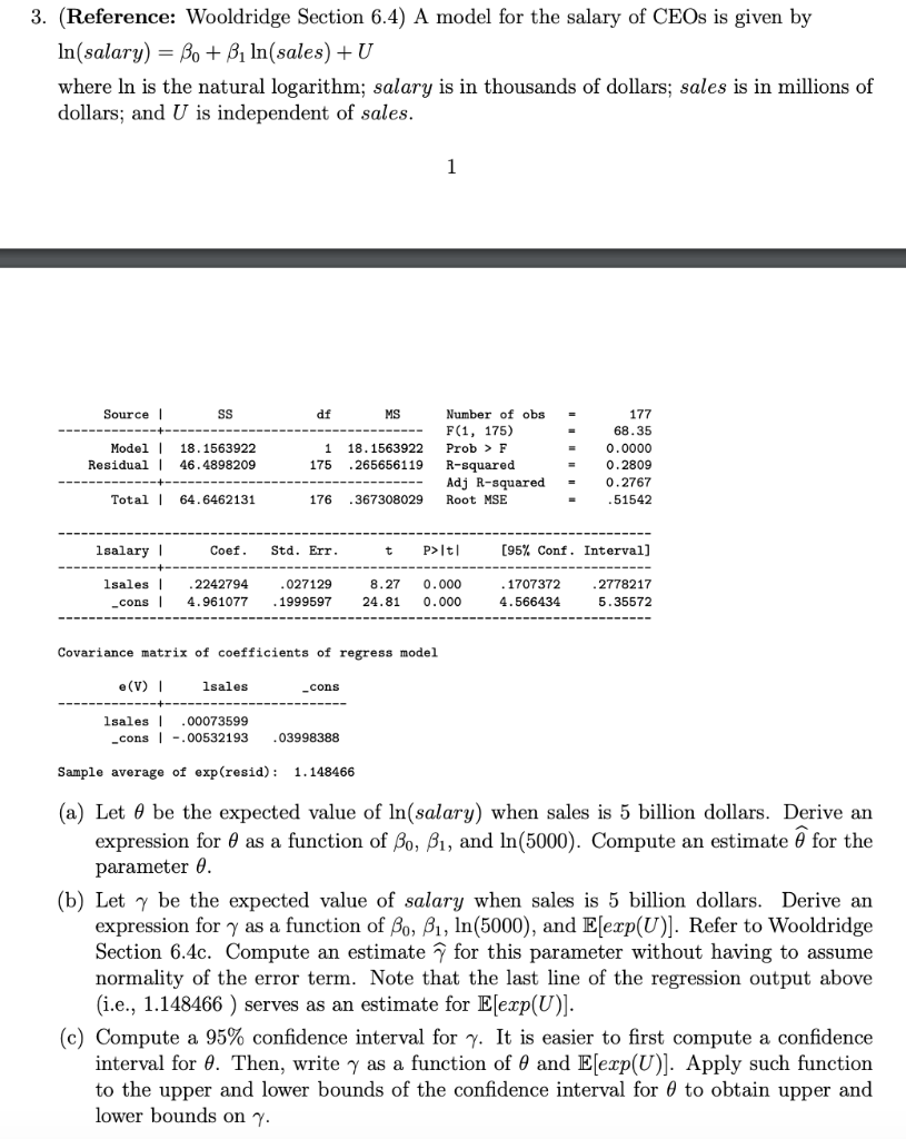
3. (Reference: Wooldridge Section 6.4) A model for the salary of CEOs is given by In(salary) = Bo + B. In(sales) +U where In is the natural logarithm; salary is in thousands of dollars; sales is in millions of dollars; and U is independent of sales. 1 Source SS df MS Model 1 Residual 18. 1563922 46.4898209 1 175 18.1563922 .265656119 Number of obs F(1, 175) Prob > F R-squared Adj R-squared Root MSE 177 68.35 0.0000 0.2809 0.2767 .51542 Total 64.6462131 176 .367308029 lsalary Coef. Std. Err P>It! (95% Conf. Interval] Isales | _cons .2242794 4.961077 .027129 . 1999597 0.000 8.27 24.81 0.000 1707372 4.566434 2778217 5.35572 Covariance matrix of coefficients of regress model (V) lsales cons lsales | .00073599 _cons -.00532193 .03998388 Sample average of exp(resid): 1.148466 (a) Let 6 be the expected value of In(salary) when sales is 5 billion dollars. Derive an expression for 8 as a function of Bo, B1, and In(5000). Compute an estimate @ for the parameter . (b) Let be the expected value of salary when sales is 5 billion dollars. Derive an expression for y as a function of Bo, B1, ln(5000), and E[exp(U)]. Refer to Wooldridge Section 6.4c. Compute an estimate for this parameter without having to assume normality of the error term. Note that the last line of the regression output above (i.e., 1.148466 ) serves as an estimate for E[exp(U)]. (c) Compute a 95% confidence interval for 7. It is easier to first compute a confidence interval for 6. Then, write y as a function of and Eerp(U)]. Apply such function to the upper and lower bounds of the confidence interval for @ to obtain upper and lower bounds on 7. 3. (Reference: Wooldridge Section 6.4) A model for the salary of CEOs is given by In(salary) = Bo + B. In(sales) +U where In is the natural logarithm; salary is in thousands of dollars; sales is in millions of dollars; and U is independent of sales. 1 Source SS df MS Model 1 Residual 18. 1563922 46.4898209 1 175 18.1563922 .265656119 Number of obs F(1, 175) Prob > F R-squared Adj R-squared Root MSE 177 68.35 0.0000 0.2809 0.2767 .51542 Total 64.6462131 176 .367308029 lsalary Coef. Std. Err P>It! (95% Conf. Interval] Isales | _cons .2242794 4.961077 .027129 . 1999597 0.000 8.27 24.81 0.000 1707372 4.566434 2778217 5.35572 Covariance matrix of coefficients of regress model (V) lsales cons lsales | .00073599 _cons -.00532193 .03998388 Sample average of exp(resid): 1.148466 (a) Let 6 be the expected value of In(salary) when sales is 5 billion dollars. Derive an expression for 8 as a function of Bo, B1, and In(5000). Compute an estimate @ for the parameter . (b) Let be the expected value of salary when sales is 5 billion dollars. Derive an expression for y as a function of Bo, B1, ln(5000), and E[exp(U)]. Refer to Wooldridge Section 6.4c. Compute an estimate for this parameter without having to assume normality of the error term. Note that the last line of the regression output above (i.e., 1.148466 ) serves as an estimate for E[exp(U)]. (c) Compute a 95% confidence interval for 7. It is easier to first compute a confidence interval for 6. Then, write y as a function of and Eerp(U)]. Apply such function to the upper and lower bounds of the confidence interval for @ to obtain upper and lower bounds on 7