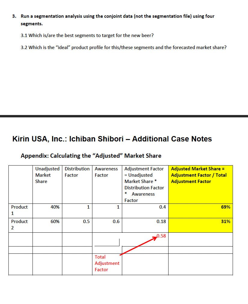
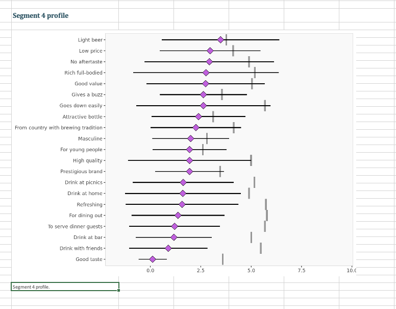
Question: 3. Run a segmentation analysis using the conjoint data (not the segmentation file) using four segments. 3.1 Which is/are the best segments to target for

3. Run a segmentation analysis using the conjoint3. Run a segmentation analysis using the conjoint3. Run a segmentation analysis using the conjoint3. Run a segmentation analysis using the conjoint3. Run a segmentation analysis using the conjoint3. Run a segmentation analysis using the conjoint3. Run a segmentation analysis using the conjoint3. Run a segmentation analysis using the conjoint3. Run a segmentation analysis using the conjoint3. Run a segmentation analysis using the conjoint3. Run a segmentation analysis using the conjoint
3. Run a segmentation analysis using the conjoint data (not the segmentation file) using four segments. 3.1 Which is/are the best segments to target for the new beer? 3.2 Which is the "ideal" product profile for this/these segments and the forecasted market share? Kirin USA, Inc.: Ichiban Shibori - Additional Case Notes Appendix: Calculating the "Adjusted" Market Share Unadjusted Distribution Awareness Adjustment Factor Adjusted Market Share = Market Factor Factor = Unadjusted Adjustment Factor / Total Share Market Share * Adjustment Factor Distribution Factor * Awareness Factor Product 40% 1 1 0.4 69% 1 Product 50% 0.5 0.6 31% 2 20.58 Tota Adjustment Factor4-segment solution The ideal number of segments is a function of statistical fit (what the data say), managerial relevance (what makes the most sense from a managerial point of view), and targetability (can the segments be easily targeted) When the three criteria do not perfectly converge, selecting the right number of segments becomes a judgment call. You have decided to perform the analysis with 4 segments. The segmentation method relies on the hierarchical clustering approach. This approach generates a dendrogram that we display next. Dendrogram The dendrogram represents the grouping process of observations into clusters. The chart reads from bottom (all initial observations are separated) to top (all observations are clustered into one unique segment). The height represents the distance between the two groups of observations being merged at each step. If two very distant groups are being merged, this will create a 'jump' in the dendrogram, indicating that it might be wise to stop the clustering process before. 140 120 100 Dendrogram. The dendrogram is a tree diagram to illustrate the arrangement of clusters produced by hierarchical clustering, and how the observations are incrementally clustered together.Scree plot The screeplot displays, for each cluster solution, a measure of within-cluster heterogeneity. If clusters group observations that are widely different (which will happen if the number of clusters is too small to capture the variability in the data), the value will be high. A good cluster solution might be where the screeplot displays an 'elbow, that is, where increasing the number of clusters beyond a certain point does not dramatically decreases within-cluster heterogeneity. The measure displayed in the screeplot is related, but not equivalent, to the distance reported in the dendrogram. 60000 - 50000 - 40000 - Scree plot. The scree plot compares the sum of squared error (SSE] for each cluster solution. A good cluster solution might be when the SSE slows dramatically, creating an 'elbow'. Such elbow does not always exist. From a statistical point of view, the SSE reported in the screeplot is computed as the sum of squared error between each observation and its cluster centroid (or centerl, summed over all the observations.Segment size Segment size Population Segment 1 Size Segment 2 Segment ] 317 Segment 4 87 Relative size 75 101 100% 54 249 329 179 Segment description Segment description Average val nation variable, overall for each segment (centroid). Segmentation variables that are statistically different from the rest of the population are highlighted in red (lower) or green (higher). Population Segment 1 Rich full-bodied Segment 2 4.77 Segment 3 Segment 4 3.10 Light beer 4.59 7.41 3.72 2.76 2.84 No aftertaste 4.40 4.11 4.56 3.82 3.48 Refreshing 5.25 5.56 5.02 5.41 2.93 Goes down easily 431 7.06 5.17 1.57 4.85 Gives a buzz 5.45 6.58 3.39 2 63 3.33 Good taste 3.48 3.79 3.000 2.63 1 069 Low price 0.120 8.347 191 0.111 3.22 Good value 437 4.67 4.65 2.96 4.76 From country with brewing tradition 4.45 5.72 3.82 2.74 3.82 Attractive bottle 4.29 4.30 100 2.26 3.16 Prestigious brand 2.95 3.22 2.39 .20 3.13 High quality 3.32 3.84 4.476 1.94 1.678 Drink at picnics 6.680 7.465 4.56 1.944 4.89 Masculine 5.43 5.22 267 2.63 1.63 2.29 For young people 3.34 2.00 2.49 2.32 2.29 Drink with friends 3.07 1.94 4.697 4.563 6.227 Drink at home 5.713 4.34 0.889 3.26 5.44 To serve dinner guests 5.90 4.92 1 61 4.37 6.24 For dining out 6.40 1.20 5.03 5.08 5.99 Drink at bar 6.24 1.37 4.35 4.62 4.99 5.34 1.17 Statistical differences in profiles Rich full-bodied - Light beer - No aftertaste - Refreshing - Goes down easily - Gives a buzz- Good taste- Low price - Good value - From country with brewing tradition - Lower (p.<.05 attractive bottle lower n.5. prestigious brand higher high quality drink at picnics masculine for young people with friends home to serve dinner guests dining out bar- segment differences per segment. cell colors indicate what extent a is statistically different from the rest of population on each segmentation variable.spider chart spider comparing averages variables across all segments. barkich full-bodied light beer no aftertaste refreshing nk goes down gas gives buz good taste low price value branfrom country brewing tradition i chart.segment profile following charts represent these are only available when data not standardized hence model assumes that use same scale. ordered in decreasing order magnitude. colored dots average horizontal lines standard deviations within vertical gray after excluding members under scrutiny. refreshing- easily bar friends- buzz- rich profile.segment guests- out- picnics- beer- buzz d.0 .5 profiledescriptors this table reports descriptor more can be found easier it will predict membership based descriptors alone. overall and cluster. highlighted red or green weekly consumption age income education sex adapt new situation make .23 do like tied timetable take chances travel abroad ethnic food knowledgeable about statistical situations- distribution populationintroduction often customer may managers but customers available. section we explore whether alone sufficient accuracy. confusion matrix hit rates below accurate enough. member classification enginius uses multinomial logit one used between multiple alternatives predictive modeling module. largest selected as default option identifies which most significant predicting cluster memberships. if highly its p-values close zero cells appear coefficients parameters baseline d.152 situations .140 probabilities parameter estimates by chance. j.482 .650 d.747 .48 d.054>

Step by Step Solution

There are 3 Steps involved in it

1 Expert Approved Answer
Step: 1 Unlock blur-text-image
Question Has Been Solved by an Expert!

Get step-by-step solutions from verified subject matter experts

Step: 2 Unlock
Step: 3 Unlock

Students Have Also Explored These Related Mathematics Questions!