4.16 Chapter 4 HW - Spreadsheet Mastery Please fill in the empty squares outlined/boxed in black. too see the images clearer, please right click and "open image in new tab." thank you!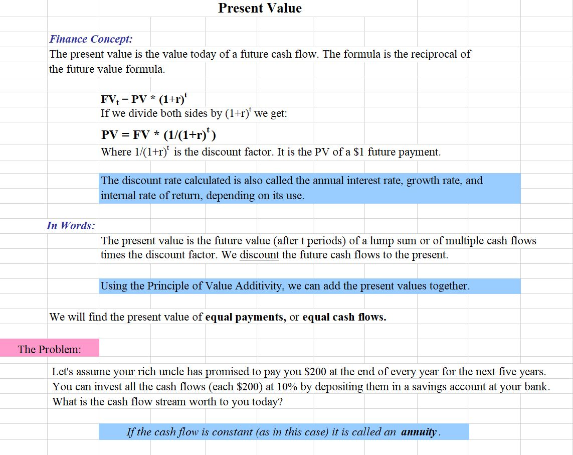

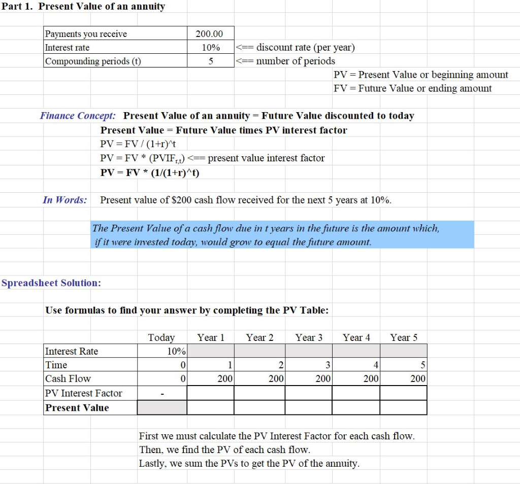
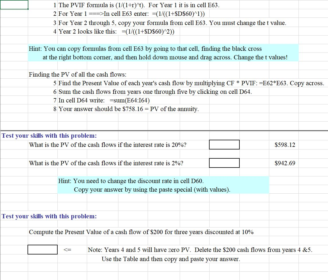
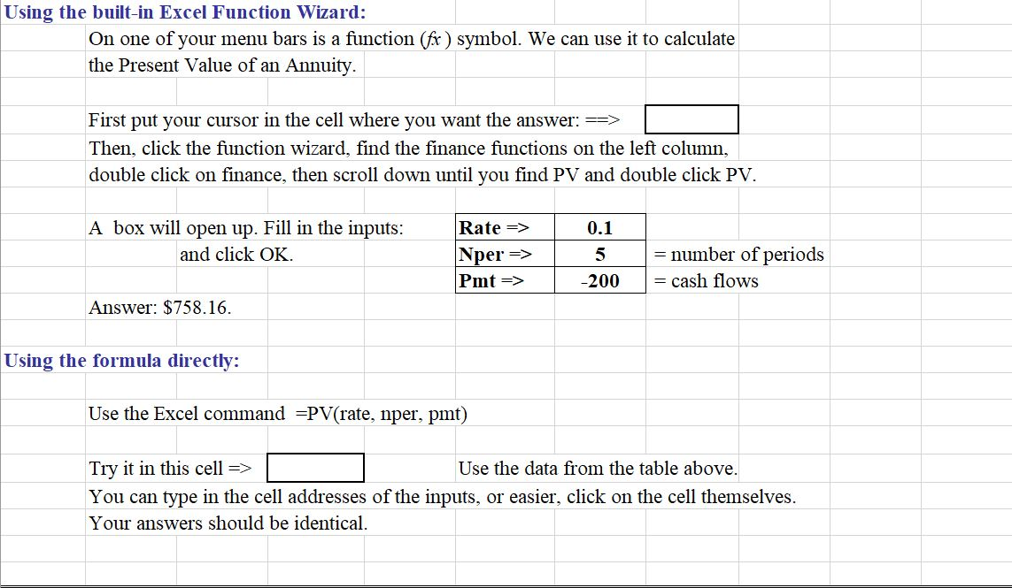
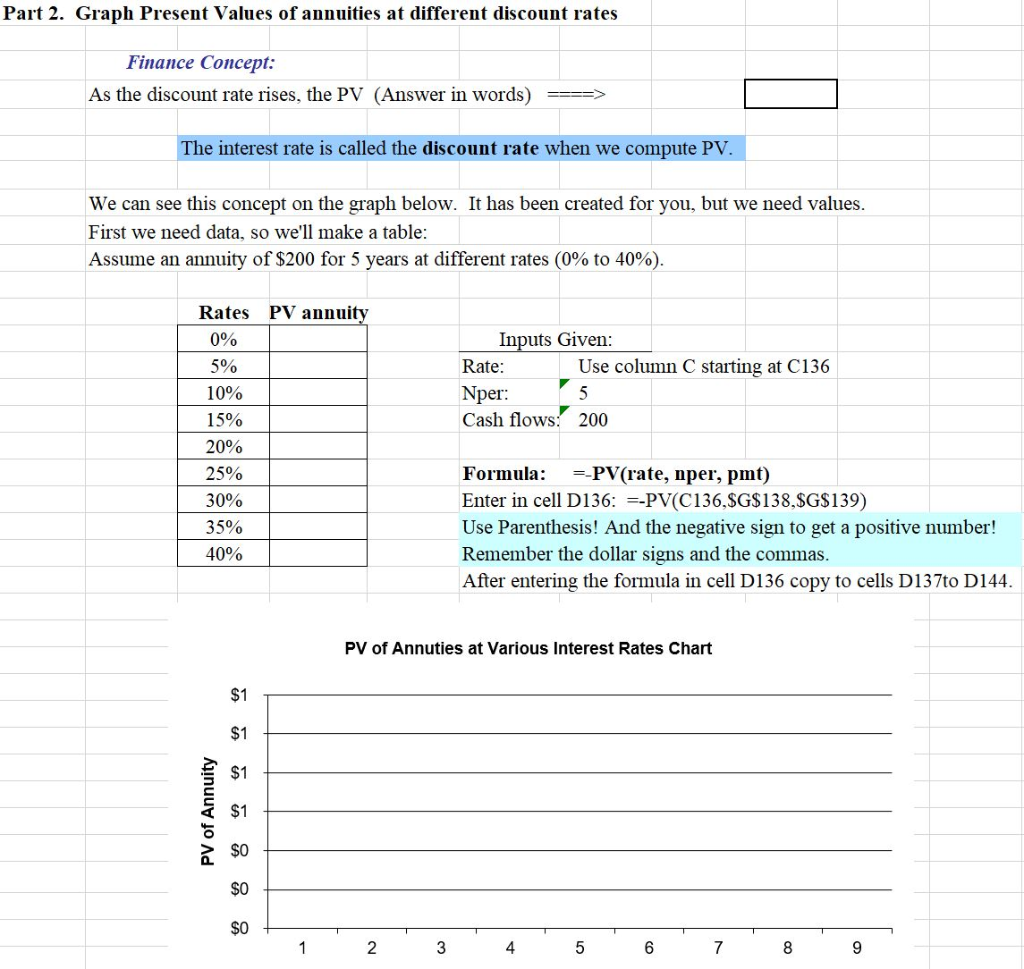
Present Value Finance Concept: The present value is the value today of a future cash flow. The formula is the reciprocal of the future value formula. FV = PV * (1+r) If we divide both sides by (1+r)' we get: PV = FV * (1/(1+r)) Where 1/(1+r) is the discount factor. It is the PV of a $1 future payment. The discount rate calculated is also called the annual interest rate, growth rate, and internal rate of return, depending on its use. In Words: The present value is the future value (after t periods) of a lump sum or of multiple cash flows times the discount factor. We discount the future cash flows to the present. Using the Principle of Value Additivity, we can add the present values together. We will find the present value of equal payments, or equal cash flows. The Problem: Let's assume your rich uncle has promised to pay you $200 at the end of every year for the next five years. You can invest all the cash flows (each $200) at 10% by depositing them in a savings account at your bank. What is the cash flow stream worth to you today? If the cash flow is constant (as in this case) it is called an annuity. Part 1. Present Value of an annuity Payments you receive Interest rate Compounding periods (t) 200.00 10% 5 In cell E63 enter: =(1/((1+$D$60)^1)) 3 For Year 2 through 5, copy your formula from cell E63. You must change the t value. 4 Year 2 looks like this: =(1/((1+$D$60)^2)) Hint: You can copy formulas from cell E63 by going to that cell, finding the black cross at the right bottom corner, and then hold down mouse and drag across. Change the t values! Finding the PV of all the cash flows: 5 Find the Present Value of each year's cash flow by multiplying CF * PVIF: =E62*E63. Copy across. 6 Sum the cash flows from years one through five by clicking on cell D64. 7 In cell D64 write: =sum(E64:164) 8 Your answer should be $758.16 = PV of the annuity. Test your skills with this problem: What is the PV of the cash flows if the interest rate is 20%? $598.12 What is the PV of the cash flows if the interest rate is 2%? $942.69 Hint: You need to change the discount rate in cell D60. Copy your answer by using the paste special (with values). Test your skills with this problem: Compute the Present Value of a cash flow of $200 for three years discounted at 10% Note: Years 4 and 5 will have zero PV. Delete the $200 cash flows from years 4 &5. Use the Table and then copy and paste your answer. Using the built-in Excel Function Wizard: On one of your menu bars is a function (fx ) symbol. We can use it to calculate the Present Value of an Annuity. First put your cursor in the cell where you want the answer: ==> Then, click the function wizard, find the finance functions on the left column, double click on finance, then scroll down until you find PV and double click PV. A box will open up. Fill in the inputs: and click OK. Rate => Nper Pmt => 0.1 5 -200 = number of periods = cash flows Answer: $758.16. Using the formula directly: Use the Excel command =PV(rate, nper, pmt) Try it in this cell => Use the data from the table above. You can type in the cell addresses of the inputs, or easier, click on the cell themselves. Your answers should be identical. Part 2. Graph Present Values of annuities at different discount rates Finance Concept: As the discount rate rises, the PV (Answer in words) The interest rate is called the discount rate when we compute PV. We can see this concept on the graph below. It has been created for you, but we need values. First we need data, so we'll make a table: Assume an annuity of $200 for 5 years at different rates (0% to 40%). Inputs Given: Rate: Use column C starting at C136 Nper: 5 Cash flows: 200 Rates PV annuity 0% 5% 10% 15% 20% 25% 30% 35% 40% Formula: =-PV(rate, nper, pmt) Enter in cell D136: -PV(C136,$G$138,$G$139) Use Parenthesis! And the negative sign to get a positive number! Remember the dollar signs and the commas. After entering the formula in cell D136 copy to cells D137to D144. PV of Annuties at Various Interest Rates Chart $1 $1 PV of Annuity $0 $0 1 2 3 4 5 6 7 8 9 The chart fills in automatically. It is made by the chart function in Excel. You can change any of the inputs and the chart will adjust automatically. Note: As interest rates increase, the PV of the annuity decreases, an inverse relationship