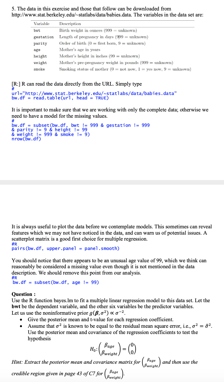
5. The data in this exercise and those that follow can be downloaded from http://www.stat.berkeley.edu/~statlabs/data/babies.data. The variables in the data set are: Variable Description but Birth weight in ounces (999 = unknown) gestation Length of pregnancy in days (909 = unknown) parity Order of birth (0 = first born, 9 = unknown) age Mother's age in years height Mother's height in inches (99 = unknown) weight Mother's pre-pregnancy weight in pounds (999 = unknown) smoke Smoking status of mother (0 = not now, 1 = yes now, 9 = unknown) [R:] R can read the data directly from the URL. Simply type # url="http://www.stat.berkeley. edu/~statlabs/data/babies. data" bw. df = read. table (url, head = TRUE) It is important to make sure that we are working with only the complete data; otherwise we need to have a model for the missing values. # bw. df = subset (bw. df, bwt != 999 & gestation != 999 & parity != 9 & height != 99 & weight != 999 & smoke != 9) nrow(bw . df) It is always useful to plot the data before we contemplate models. This sometimes can reveal features which we may not have noticed in the data, and can warn us of potential issues. A scatterplot matrix is a good first choice for multiple regression. # R pairs (bw. df, upper . panel = panel . smooth) You should notice that there appears to be an unusual age value of 99, which we think can reasonably be considered a missing value even though it is not mentioned in the data description. We should remove this point from our analysis. # R bw. df = subset(bw. df, age != 99) Question : Use the R function bayes.Im to fit a multiple linear regression model to this data set. Let the but be the dependent variable, and the other six variables be the predictor variables. Let us use the noninformative prior g (B, 62) oco-2 . Give the posterior mean and t-value for each regression coefficient. Assume that o is known to be equal to the residual mean square error, i.e., 62 = 62. Use the posterior mean and covariance of the regression coefficients to test the hypothesis Bage Ho: \\Bweight, ) = (8) Hint: Extract the posterior mean and covariance matrix for( Bage Bweight and then use the credible region given in page 43 of C7 for ( Bage (Bweight)