#5. Using PYTHON

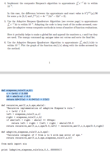
Implement the composite Simpson's algorithm to approximate integral^5_0 e^-x^2 dx to within 10^-8. In this case, the difference between the approximate and exact value is h^4 f^(4) (mu)/36 for some mu in [0, 5] and f^(4) (x) = 4e^-x (4x^4 - 12x^2 + 3). Use the Adaptive Simpson Quadrature Algorithm (see reverse page) to approximate integral^5_0 e^-x^3 dx to within 10^-8. Adapting the code to keep track of the nodes accessed, compare the adaptive versus composite methods in terms of number of function evaluations. Here it probably helps to make a global list and append the numbers a, c and b as they are used. The numpy command np.unique takes out extras and sorts the final list. Use the Adaptive Simpson Quadrature Algorithm to approximate integral^2_0.1 sin(1/x) dx to within 10^-3. Plot the graph of the function sin(1/x) along with the nodes accessed by the method. def Simpsons_rule (f, a, b): c = (a + b)/2.000 h3 = abs (b-a)/6.0 return h3*(f(a) + 4.0*f(c) + f(b)) def recursive_asr (f, a, b, b, eps, whole): "Recursive implementation of adaptive Simpson's rule." c = (a + b)/2.0 left = simpsons_rule (f, a, c) right = Simpsons_rule(f, c, b) if abs(left + right = whole) 15 * eps: return left + right + (left + right = whole)/15.0 return recursive_asr (f, a, c, eps/2.0 left) + recursive_asr (f, c, b, eps/2.0, right) def adaptive_simpsons_rule (f, a, b, eps): "Calculate integral of f from a to b with max error of eps." return recursive_asr (f, a, b, eps, Simpsons_rule(f, a, b)) from math import sin print (adaptive_simpsons_rule (sin, 0, 1, .0000001)) Implement the composite Simpson's algorithm to approximate integral^5_0 e^-x^2 dx to within 10^-8. In this case, the difference between the approximate and exact value is h^4 f^(4) (mu)/36 for some mu in [0, 5] and f^(4) (x) = 4e^-x (4x^4 - 12x^2 + 3). Use the Adaptive Simpson Quadrature Algorithm (see reverse page) to approximate integral^5_0 e^-x^3 dx to within 10^-8. Adapting the code to keep track of the nodes accessed, compare the adaptive versus composite methods in terms of number of function evaluations. Here it probably helps to make a global list and append the numbers a, c and b as they are used. The numpy command np.unique takes out extras and sorts the final list. Use the Adaptive Simpson Quadrature Algorithm to approximate integral^2_0.1 sin(1/x) dx to within 10^-3. Plot the graph of the function sin(1/x) along with the nodes accessed by the method. def Simpsons_rule (f, a, b): c = (a + b)/2.000 h3 = abs (b-a)/6.0 return h3*(f(a) + 4.0*f(c) + f(b)) def recursive_asr (f, a, b, b, eps, whole): "Recursive implementation of adaptive Simpson's rule." c = (a + b)/2.0 left = simpsons_rule (f, a, c) right = Simpsons_rule(f, c, b) if abs(left + right = whole) 15 * eps: return left + right + (left + right = whole)/15.0 return recursive_asr (f, a, c, eps/2.0 left) + recursive_asr (f, c, b, eps/2.0, right) def adaptive_simpsons_rule (f, a, b, eps): "Calculate integral of f from a to b with max error of eps." return recursive_asr (f, a, b, eps, Simpsons_rule(f, a, b)) from math import sin print (adaptive_simpsons_rule (sin, 0, 1, .0000001))