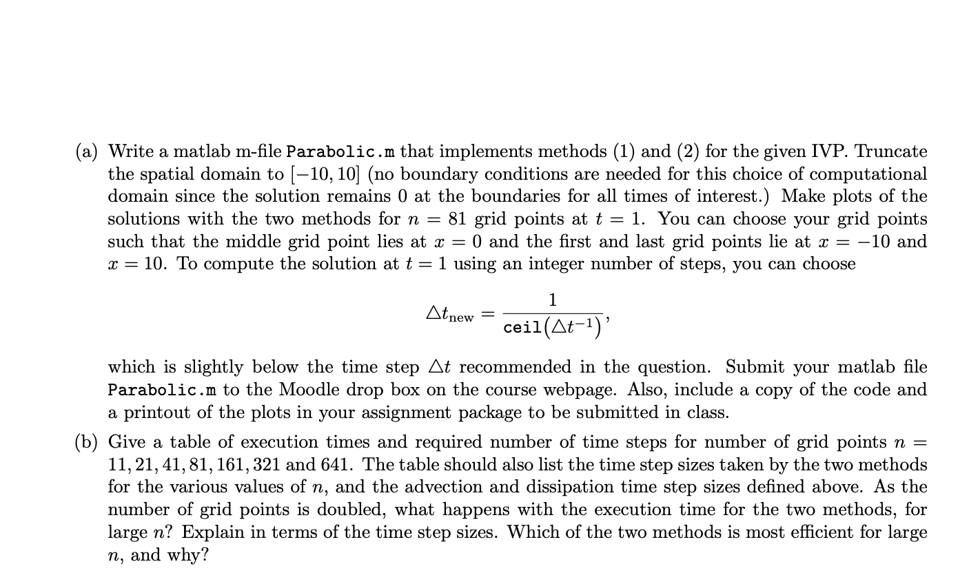
Question: 6. Finite Difference Method for 2D Elliptic PDEs (20 marks). (a) Implement a Matlab function with header function A=build laplace 2D (m) that constructs a


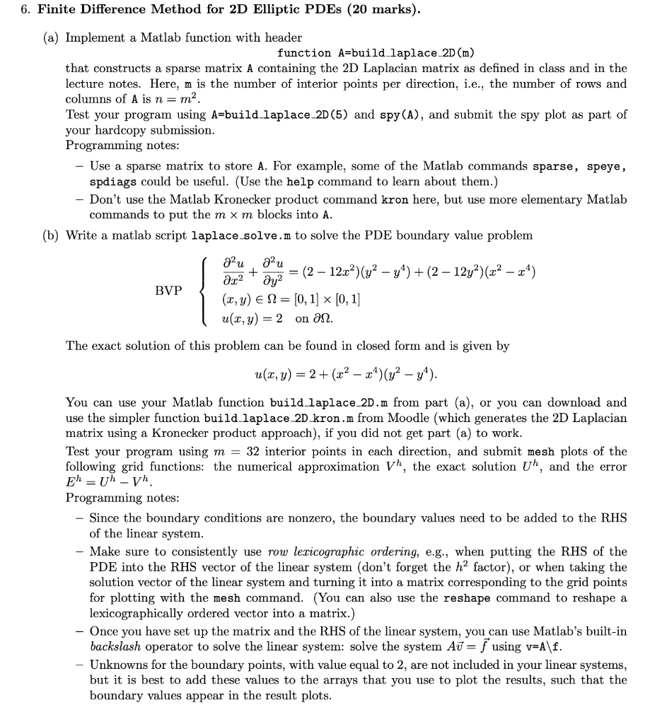
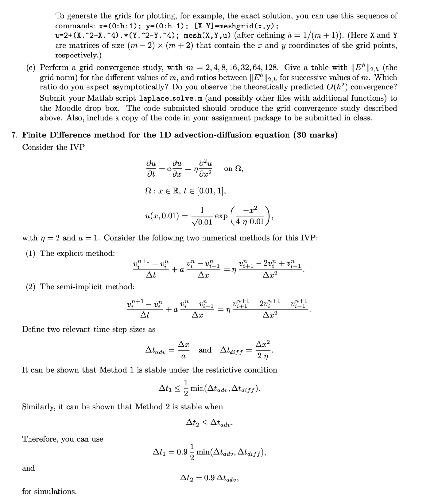
6. Finite Difference Method for 2D Elliptic PDEs (20 marks). (a) Implement a Matlab function with header function A=build laplace 2D (m) that constructs a sparse matrix A containing the 2D Laplacian matrix as defined in class and in the lecture notes. Here, m is the number of interior points per direction, i.e., the number of rows and columns of A is n = m2. Test your program using A=build laplace 2D (5) and spy(A), and submit the spy plot as part of your hardcopy submission. Programming notes: - Use a sparse matrix to store A. For example, some of the Matlab commands sparse, speye, spdiags could be useful. (Use the help command to learn about them.) Don't use the Matlab Kronecker product command kron here, but use more elementary Matlab commands to put the m x m blocks into (b) Write a matlab script laplace-solve.m to solve the PDE boundary value problem BVP { a2u ? + = (2 12.0?)(y2 44) + (2 12y?)(x2 x4) ar2 ay2 (x, y) EN = [0, 1] x [0, 1] u(x, y) = 2 on an. The exact solution of this problem can be found in closed form and is given by u(x, y) = 2 + (x2 x^)(y2 y^). You can use your Matlab function build laplace 2D.m from part (a), or you can download and use the simpler function build laplace 2D kron.m from Moodle (which generates the 2D Laplacian matrix using a Kronecker product approach), if you did not get part (a) to work. Test your program using m = 32 interior points in each direction, and submit mesh plots of the following grid functions: the numerical approximation Vh, the exact solution Uh, and the error Eh = Uh - vh Programming notes: Since the boundary conditions are nonzero, the boundary values need to be added to the RHS of the linear system. Make sure to consistently use row lexicographic ordering, e.g., when putting the RHS of the PDE into the RHS vector of the linear system (don't forget the ha factor), or when taking the solution vector of the linear system and turning it into a matrix corresponding to the grid points for plotting with the mesh command. (You can also use the reshape command to reshape a lexicographically ordered vector into a matrix.) - Once you have set up the matrix and the RHS of the linear system, you can use Matlab's built-in backslash operator to solve the linear system: solve the system A= using v=A\f. Unknowns for the boundary points, with value equal to 2, are not included in your linear systems, but it is best to add these values to the arrays that you use to plot the results, such that the boundary values appear in the result plots. To generate the grids for plotting, for example, the exact solution, you can use this sequence of commands: x=(0:h:1); y=(0:h:1); [X Y] =meshgrid(x,y); u=2+(x.^2-x. 4).*(Y. 2-Y. 4); mesh(X,Y,u) (after defining h = 1/(m +1)). (Here X and Y are matrices of size (m+2) x (m+2) that contain the r and y coordinates of the grid points, respectively.) (c) Perform a grid convergence study, with m = 2,4,8, 16, 32, 64, 128. Give a table with ||E" ||2,1 (the grid norm) for the different values of m, and ratios between |E ||2,n for successive values of m. Which ratio do you expect asymptotically? Do you observe the theoretically predicted (ha) convergence? Submit your Matlab script laplace_solve.m (and possibly other files with additional functions) to the Moodle drop box. The code submitted should produce the grid convergence study described above. Also, include a copy of the code in your assignment package to be submitted in class. 7. Finite Difference method for the 1D advection-diffusion equation (30 marks) Consider the IVP au au + a at ar 1ac on , 12:7 ER, t (0.01, 1], exp la 4 whti ta 1 u(x,0.01) = 0.01 0.01 with n= 2 and a = 1. Consider the following two numerical methods for this IVP: (1) The explicit method: :- - U1 v+1 -20 + 1 = AC A22 (2) The semi-implicit method: -20%+1 +0,"+1 + a n At Ar2 Define two relevant time step sizes as AC Ar2 Atadu = and Atdiff = a Un+1 - 0 211 It can be shown that Method 1 is stable under the restrictive condition Atz 55 min(Atadu, Atdiss). Similarly, it can be shown that Method 2 is stable when Atz
Step by Step Solution
There are 3 Steps involved in it

Get step-by-step solutions from verified subject matter experts


